A Usage Template for the R Package msDiaLogue
Shiying Xiao, Charles Watt, Jennifer C. Liddle, Jeremy L. Balsbaugh, Timothy E. Moore
Department
of Statistics, UConn
Proteomics
and Metabolomics Facility, UConn
Statistical
Consulting Services, UConn
2025-06-11
Source:vignettes/usage_template.Rmd
usage_template.RmdPreprocessing
Usage
preprocessing(
  fileName,            # name of Spectronaut file
  dataSet = NULL,      # name of dataset if already loaded into R
  filterNaN = TRUE,    # Should NaN values be removed?
  filterUnique = 2,    # Minimum number of unique peptides
  replaceBlank = TRUE, # Replace blank protein names with Accession num.
  saveRm = TRUE        # Should excluded proteins be saved to a file?
)
Details & Examples
The function preprocessing() takes a .csv
file of summarized protein abundances, exported from
Spectronaut. The most important columns that need to be
included in this file are: R.Condition,
R.Replicate, PG.ProteinAccessions,
PG.ProteinNames,
PG.NrOfStrippedSequencesIdentified, and
PG.Quantity. This function will reformat the data and
provide functionality for some initial filtering (based on the number of
unique peptides). The steps below describe the functions that happen in
the Preprocessing code.
1. Loads the raw data
If the raw data is in a .csv file Toy_Spectronaut_Data.csv, specify the
fileNameto read the raw data file into R.If the raw data is stored as an .RData file Toy_Spectronaut_Data.RData, first load the data file directly, then specify the
dataSetin the function.
2. Filters out identified proteins that exhibit “NaN” quantitative values
NaN, which stands for ‘Not a Number,’ can be found in the PG.Quantity column for proteins that were identified by MS and MS/MS evidence in the raw data, but all peptides from that protein lack an associated integrated peak area or intensity. This usually occurs in low abundance peptides that exhibit intensities close to the limit of detection resulting in poor signal-to-noise (S/N) and/or when there is interference from other co-eluting peptide ions with very similar or identical m/z values that lead to difficulty in parsing out individual intensity profiles.
3. Applies a unique peptides per protein filter
General practice in the proteomics field is to filter out proteins which were identified on the basis of a single peptide. Because approximately 1% of all identified peptides are false positive matches, it’s more likely that 1 peptide was incorrectly identified and that protein ID is incorrect than that, for example, 5 peptides from the same protein were all incorrectly identified and that protein ID is incorrect. We recommend focusing on proteins with 2 or more peptide identifications, as these will be higher confidence. If you have a protein of interest with only 1 peptide identified, contact PMF faculty and we can help you evaluate the evidence from the raw data to determine believability.
4. Adds accession numbers to identified proteins without informative names
Spectronaut reports contain 4 different columns of identifying information:
-
PG.Genes, which is the gene name (e.g. CDK1). -
PG.ProteinAccessions, which is the UniProt identifier number for a unique entry in the online database (e.g. P06493). -
PG.ProteinDescriptions, which is the protein name as provided on UniProt (e.g. cyclin-dependent kinase 1). -
PG.ProteinNames, which is a concatenation of an identifier and the species (e.g. CDK1_HUMAN).
Every entry in UniProt will have an accession number, but may not
have all of the other identifiers, due to incomplete annotation. Because
Uniprot includes entries for fragments of proteins and some proteins
entries are redundant, a peptide can match to multiple entries for the
same protein, which generates multiple possible identifiers in
Spectronaut. Further, the ProteinNames
entry in Spectronaut can switch formats: the preference
is accession number and species, but can also be gene name and species
instead.
This option tells msDiaLogue to substitute the accession number for an identifier if it tries to pull an identifier from a column with no information.
5. Saves a document to your working directory with all filtered out data, if desired
If saveRm = TRUE, the data removed in step 2
(preprocess_Filtered_Out_NaN.csv) and step 3
(preprocess_Filtered_Out_Unique.csv) will be saved in the
current working directory.
As part of the preprocessing(), a histogram of
-transformed
protein abundances is provided. This is a helpful way to confirm that
the data have been read in correctly, and there are no issues with the
numerical values of the protein abundances. Ideally, this histogram will
appear fairly symmetrical (bell-shaped) without too much skew towards
smaller or larger values.
## if the raw data is in a .csv file
fileName <- "../tests/testData/Toy_Spectronaut_Data.csv"
dataSet <- preprocessing(fileName,
                         filterNaN = TRUE, filterUnique = 2,
replaceBlank = TRUE, saveRm = TRUE)preprocessing() does not perform a
transformation on your data. You still need to use the function
transform().
## if the raw data is in an .Rdata file
load("../tests/testData/Toy_Spectronaut_Data.RData")
dataSet <- preprocessing(dataSet = Toy_Spectronaut_Data,
                         filterNaN = TRUE, filterUnique = 2,
                         replaceBlank = TRUE, saveRm = TRUE)
#> Warning: Removed 62 rows containing non-finite outside the scale range
#> (`stat_bin()`).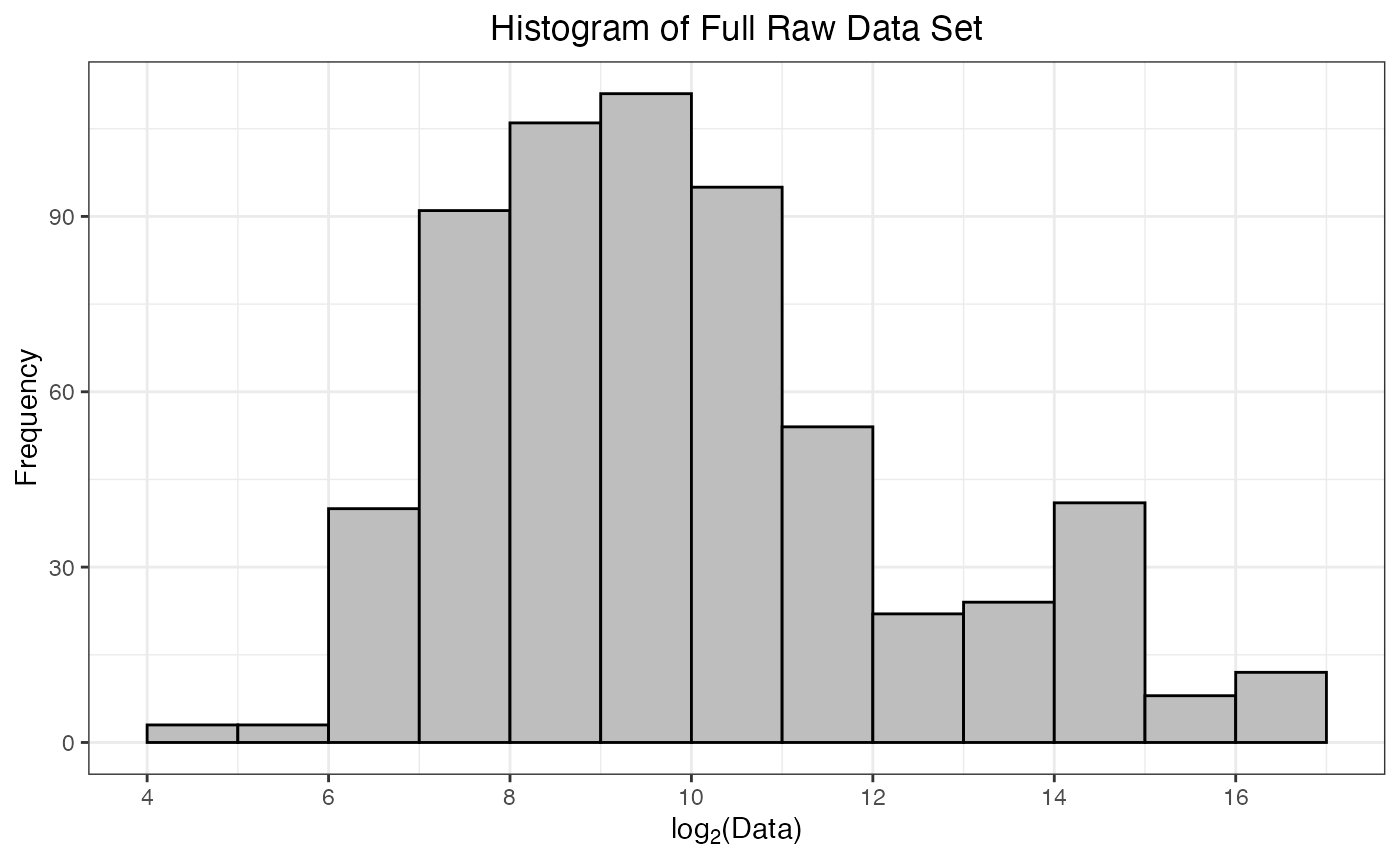
#> Summary of Full Data Signals (Raw):
#>      Min.   1st Qu.    Median      Mean   3rd Qu.      Max.
#>     20.93    263.87    669.79   6897.92   1963.53 117803.49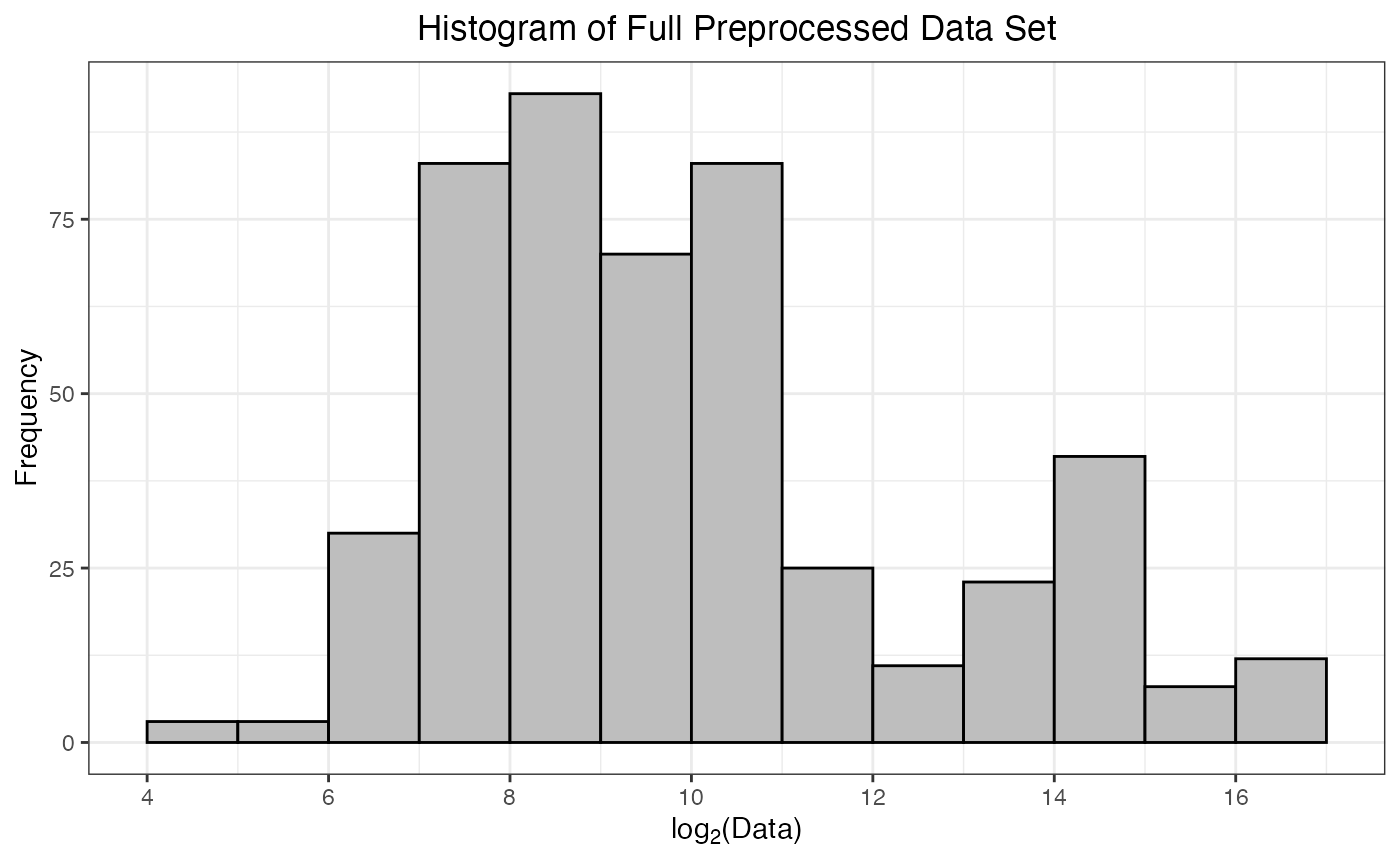
#> Levels of Condition: 100pmol 200pmol 50pmol
#> Levels of Replicate: 1 2 3 4| R.Condition | R.Replicate | NUD4B_HUMAN | A0A7P0T808_HUMAN | A0A8I5KU53_HUMAN | ZN840_HUMAN | CC85C_HUMAN | TMC5B_HUMAN | C9JEV0_HUMAN | C9JNU9_HUMAN | ALBU_BOVIN | CYC_BOVIN | TRFE_BOVIN | KRT16_MOUSE | F8W0H2_HUMAN | H0Y7V7_HUMAN | H0YD14_HUMAN | H3BUF6_HUMAN | H7C1W4_HUMAN | H7C3M7_HUMAN | TCPR2_HUMAN | TLR3_HUMAN | LRIG2_HUMAN | RAB3D_HUMAN | ADH1_YEAST | LYSC_CHICK | BGAL_ECOLI | CYTA_HUMAN | KPCB_HUMAN | LIPL_HUMAN | PIP_HUMAN | CO6_HUMAN | BGAL_HUMAN | SYTC_HUMAN | CASPE_HUMAN | DCAF6_HUMAN | DALD3_HUMAN | HGNAT_HUMAN | RFFL_HUMAN | RN185_HUMAN | ZN462_HUMAN | ALKB7_HUMAN | POLK_HUMAN | ACAD8_HUMAN | A0A7I2PK40_HUMAN | NBDY_HUMAN | H0Y5R1_HUMAN |
|---|---|---|---|---|---|---|---|---|---|---|---|---|---|---|---|---|---|---|---|---|---|---|---|---|---|---|---|---|---|---|---|---|---|---|---|---|---|---|---|---|---|---|---|---|---|---|
| 100pmol | 1 | 1547.983 | 3168.32568 | 2819.7874 | 318.54376 | 495.5136 | 456.3309 | 213.21727 | 237.1306 | 111209.7 | 10737.953 | 15097.67 | 1799.391 | 630.1937 | 1311.8127 | 1279.6390 | 280.6318 | 299.51523 | 1154.5566 | 16461.2012 | 179.3190 | 516.1104 | 1234.587 | 27599.42 | 13798.590 | 23840.03 | 614.0895 | 990.5613 | 440.0417 | 132.31737 | 150.6033 | 3578.014 | 26872.50 | 109.55331 | 211.6450 | 1292.5234 | 1963.5321 | 189.79155 | 1106.1482 | 981.11432 | 180.6320 | 199.14555 | 209.7806 | NA | NA | NA |
| 100pmol | 2 | 1680.730 | 4576.37158 | 1061.9502 | 404.25836 | 556.8611 | 501.0473 | 184.89574 | 314.0320 | 111659.9 | 10655.384 | 15840.28 | NA | 575.0490 | 1114.2773 | 1294.9751 | 271.8160 | 248.04329 | 1032.0381 | 1460.7496 | 213.1137 | 492.3771 | 1186.433 | 27221.59 | 13880.411 | 23963.31 | 640.2153 | 1077.4829 | 364.5241 | 128.78983 | 128.2592 | 3412.794 | 26742.22 | 155.37483 | 348.6104 | 1066.3511 | 1509.1512 | 153.90802 | 1303.6520 | 388.65823 | 122.7458 | 751.19849 | 247.3832 | 1420.1351 | NA | NA |
| 100pmol | 3 | 1414.811 | 4675.13281 | 2177.8496 | 275.09167 | 559.3206 | NA | 111.24314 | 501.2060 | 105982.9 | 10663.714 | 15022.21 | NA | 613.3968 | 1224.3837 | 946.0795 | 309.7599 | 270.67770 | 1808.1924 | 21555.3555 | 200.7485 | 342.1992 | 1227.435 | 26587.62 | 13723.719 | 22957.35 | 551.6828 | 1176.7791 | 319.0364 | NA | 118.5104 | 3499.113 | 26124.20 | 91.82145 | 319.1320 | 1003.3372 | 1342.4712 | 143.12419 | 1352.7024 | 430.13318 | 144.6799 | 171.13177 | 221.9161 | 1889.0665 | 835.6825 | NA |
| 100pmol | 4 | 1620.490 | 3828.19971 | 2062.8384 | 385.05573 | 558.0967 | 422.0465 | 84.27336 | 334.6389 | 104442.6 | 10843.115 | 15160.49 | NA | 886.5406 | 1148.7343 | 1091.7800 | NA | 229.40149 | 901.5703 | 22937.2500 | 240.7981 | 418.1846 | 1190.952 | 26168.72 | 13944.603 | 22311.30 | 438.5425 | 1162.6656 | 351.5390 | NA | 137.8860 | 3481.821 | 25910.39 | 88.26187 | 217.7478 | 489.8084 | 1721.8601 | 99.95578 | 990.6649 | 393.55930 | 134.5238 | 145.17339 | 216.3736 | 1610.2407 | 950.3087 | 913.3416 |
| 200pmol | 1 | 1512.770 | 4232.05078 | 2004.8613 | 338.27777 | 156.3478 | 364.5416 | 146.80331 | NA | 109245.3 | 19524.863 | 21577.97 | 2212.190 | 491.7787 | 1246.4460 | 1080.4132 | 270.1487 | 252.09808 | 1454.3271 | 21113.4512 | 223.8396 | 313.7860 | 1176.982 | 48693.35 | 24344.188 | 41234.67 | 364.7307 | 1203.0853 | 385.5154 | 65.40555 | 151.0895 | 3553.484 | 26261.47 | 81.22160 | 185.4865 | 939.8899 | 2149.7632 | 131.13179 | 381.0588 | 429.62201 | 239.4998 | 145.04378 | 424.7914 | 2337.8496 | NA | 837.8737 |
| 200pmol | 2 | 1480.490 | 3496.84155 | 2177.9534 | NA | 550.4083 | NA | 135.78349 | 295.8571 | 113357.5 | 20072.297 | 22968.96 | NA | 669.7894 | 1068.2001 | NA | 285.4891 | 259.50000 | 1049.7526 | 25760.0527 | 190.3054 | 452.8294 | 1220.266 | 49866.29 | 24742.227 | 42899.43 | 633.5656 | 1234.5601 | 414.1271 | NA | 135.8605 | 3686.869 | 27638.89 | 69.56509 | 250.4035 | 1020.4291 | 725.6615 | 116.20615 | 877.0164 | 438.22589 | 133.4297 | 160.92671 | 155.0986 | NA | 1053.8444 | 1000.5491 |
| 200pmol | 3 | 1555.834 | 356.43225 | 2280.6846 | 379.62103 | 564.2863 | 496.0772 | 103.30424 | 473.9141 | 114321.8 | 20787.127 | 20720.13 | 1451.198 | 586.7260 | 1378.0652 | 1194.8448 | 291.6754 | 184.18954 | 1123.7469 | NA | 174.5702 | 432.1681 | 1216.306 | 50704.73 | 24803.633 | 42904.95 | 446.4135 | 1082.7312 | 357.6343 | NA | 129.0676 | 3530.710 | 27101.22 | 62.08423 | 136.7023 | 1171.5715 | 1675.6870 | 109.60301 | 938.3956 | 568.89239 | 315.7039 | 146.75146 | 198.4779 | 1397.9890 | 837.2197 | 694.5791 |
| 200pmol | 4 | 1529.628 | 350.70822 | 2223.3093 | 410.82349 | 292.9041 | 522.1325 | 95.18819 | 318.4948 | 116439.8 | 19924.240 | 22153.40 | NA | 539.0703 | 923.3237 | 1115.3848 | 322.9086 | 97.65465 | 957.0436 | NA | 164.7767 | NA | 1183.197 | 53744.70 | 26381.047 | 43279.84 | 527.1628 | 1121.3438 | 342.5055 | NA | 121.3068 | 3751.769 | 27545.24 | 70.39470 | 199.2453 | 996.0696 | 1696.6189 | 125.31519 | 611.6407 | 506.49115 | 204.4332 | 161.96100 | 376.5362 | 895.9138 | NA | NA |
| 50pmol | 1 | 1480.210 | 561.38837 | 189.9275 | 264.24271 | 308.9420 | NA | 599.90497 | 192.3859 | 117803.5 | 6758.298 | 12183.81 | NA | 594.8999 | 899.5010 | 1163.1122 | 291.4431 | 176.21545 | 620.2048 | 14107.1250 | 152.5492 | 292.2440 | 1186.543 | 16408.28 | 7169.955 | 14728.67 | 2984.7190 | 1029.7336 | 288.4770 | 891.24725 | 129.7482 | 3547.950 | 25668.78 | 846.95880 | 146.3040 | NA | 461.3821 | 86.84789 | 373.6308 | 49.93938 | 236.2902 | 20.92994 | 142.3466 | NA | NA | NA |
| 50pmol | 2 | 1486.144 | NA | 1462.2559 | 325.74991 | 351.2331 | NA | 254.75084 | 308.6775 | 110086.7 | 6721.135 | 12521.78 | NA | 582.8912 | 531.7106 | 1119.5256 | 287.1180 | 103.58258 | 849.2368 | 24912.3613 | 140.6493 | 362.3117 | 1260.574 | 16444.63 | 7797.536 | 14736.71 | 857.5026 | NA | 361.4482 | 179.10303 | 166.8891 | 3530.004 | 26351.25 | 207.83086 | 165.6463 | 265.2173 | 1184.9562 | 93.91448 | 768.2026 | 489.40918 | 146.9422 | 88.41573 | 101.6087 | NA | NA | NA |
| 50pmol | 3 | 1468.554 | 42.51457 | 1364.9075 | 83.99377 | 296.5147 | 396.0038 | 257.78970 | 279.2477 | 105640.2 | 6172.877 | 11926.22 | 1373.660 | 569.8922 | NA | 1067.0791 | 294.0919 | 88.48861 | 738.7719 | 666.5015 | NA | NA | 1175.953 | 16618.11 | 7432.793 | 14160.20 | 916.4893 | 992.5451 | 319.6350 | 128.63672 | 120.6974 | 3458.023 | 26017.54 | 203.64948 | 132.5755 | 291.4759 | 932.9668 | 93.50905 | 547.0935 | 263.86734 | 313.0341 | 111.88376 | 85.4563 | NA | NA | NA |
| 50pmol | 4 | 1497.531 | 927.07886 | 1435.5588 | 275.60831 | 242.4643 | 425.7305 | 197.71338 | 382.4084 | 110446.0 | 6028.398 | 12021.50 | NA | NA | 593.1353 | 1302.1250 | 339.3387 | 30.13688 | 873.1840 | 15711.3106 | 142.4270 | 291.5121 | 1150.711 | 16282.51 | 7543.633 | 14758.73 | 886.7808 | 1138.6193 | NA | 152.56187 | NA | 3575.316 | 25969.99 | 190.47060 | 220.1901 | 676.8246 | 996.8993 | 31.57284 | 523.4712 | 450.08408 | 164.1874 | 143.96025 | 135.2896 | NA | NA | NA |
Transformation
Usage
transform(dataSet,        # a preprocessed dataset
          method = "log", # method of transformation
          logFold = 2,    # base value for log transformation
          root = 2)       # degree of the root for a root transformation
Details & Examples
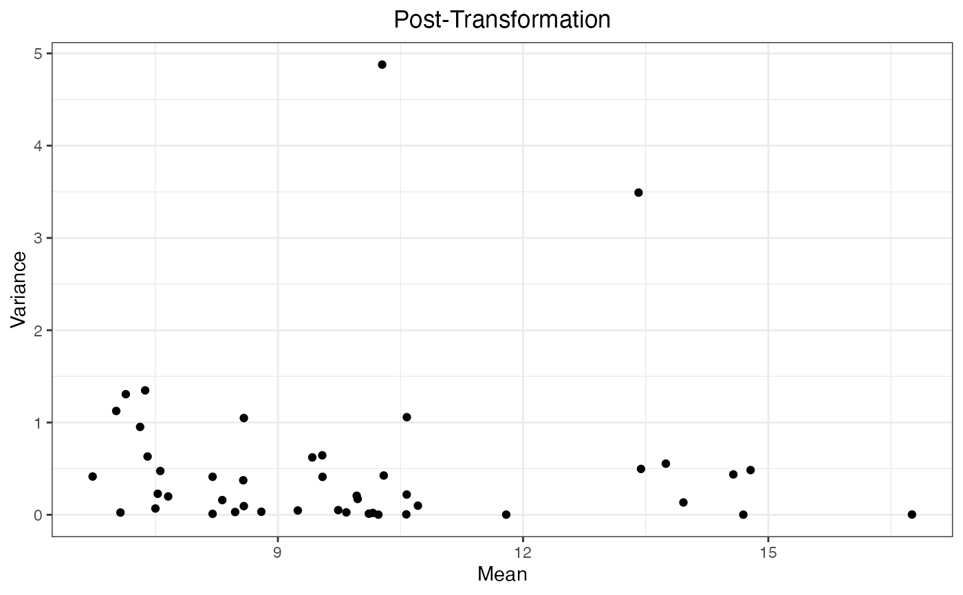
Raw mass spectrometry intensity measurements are often unsuitable for direct statistical modeling because the shape of the data is usually not symmetrical and the variance is not consistent across the range of intensities. Most proteomic workflows will convert these raw values with a log transformation, which both reshapes the data into a more symmetrical distribution, making it easier to interpret mean-based fold changes, and also stabilizes the variance across the intensity range (i.e. reduces heteroscedasticity).
dataTran <- transform(dataSet, logFold = 2)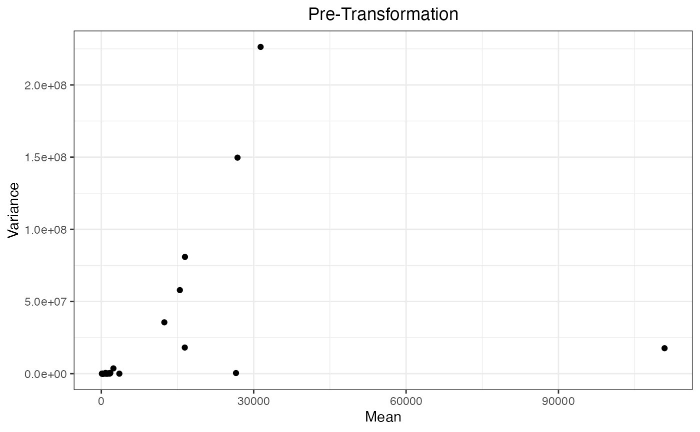
| R.Condition | R.Replicate | NUD4B_HUMAN | A0A7P0T808_HUMAN | A0A8I5KU53_HUMAN | ZN840_HUMAN | CC85C_HUMAN | TMC5B_HUMAN | C9JEV0_HUMAN | C9JNU9_HUMAN | ALBU_BOVIN | CYC_BOVIN | TRFE_BOVIN | KRT16_MOUSE | F8W0H2_HUMAN | H0Y7V7_HUMAN | H0YD14_HUMAN | H3BUF6_HUMAN | H7C1W4_HUMAN | H7C3M7_HUMAN | TCPR2_HUMAN | TLR3_HUMAN | LRIG2_HUMAN | RAB3D_HUMAN | ADH1_YEAST | LYSC_CHICK | BGAL_ECOLI | CYTA_HUMAN | KPCB_HUMAN | LIPL_HUMAN | PIP_HUMAN | CO6_HUMAN | BGAL_HUMAN | SYTC_HUMAN | CASPE_HUMAN | DCAF6_HUMAN | DALD3_HUMAN | HGNAT_HUMAN | RFFL_HUMAN | RN185_HUMAN | ZN462_HUMAN | ALKB7_HUMAN | POLK_HUMAN | ACAD8_HUMAN | A0A7I2PK40_HUMAN | NBDY_HUMAN | H0Y5R1_HUMAN |
|---|---|---|---|---|---|---|---|---|---|---|---|---|---|---|---|---|---|---|---|---|---|---|---|---|---|---|---|---|---|---|---|---|---|---|---|---|---|---|---|---|---|---|---|---|---|---|
| 100pmol | 1 | 10.59617 | 11.629505 | 11.461371 | 8.315348 | 8.952781 | 8.833937 | 7.736180 | 7.889538 | 16.76292 | 13.39043 | 13.88204 | 10.81329 | 9.299651 | 10.357346 | 10.321521 | 8.132535 | 8.226486 | 10.173123 | 14.006782 | 7.486384 | 9.011536 | 10.26981 | 14.75235 | 13.75223 | 14.54110 | 9.262305 | 9.952103 | 8.781496 | 7.047859 | 7.234610 | 11.80494 | 14.71384 | 6.775489 | 7.725502 | 10.335975 | 10.939236 | 7.568272 | 10.111329 | 9.938277 | 7.496910 | 7.637679 | 7.712738 | NA | NA | NA |
| 100pmol | 2 | 10.71487 | 12.159989 | 10.052500 | 8.659134 | 9.121174 | 8.968803 | 7.530568 | 8.294768 | 16.76875 | 13.37929 | 13.95131 | NA | 9.167541 | 10.121893 | 10.338709 | 8.086487 | 7.954448 | 10.011280 | 10.512493 | 7.735480 | 8.943620 | 10.21241 | 14.73246 | 13.76076 | 14.54854 | 9.322413 | 10.073449 | 8.509870 | 7.008875 | 7.002919 | 11.73674 | 14.70683 | 7.279609 | 8.445472 | 10.058467 | 10.559522 | 7.265925 | 10.348343 | 8.602358 | 6.939530 | 9.553050 | 7.950604 | 10.471813 | NA | NA |
| 100pmol | 3 | 10.46639 | 12.190792 | 11.088689 | 8.103769 | 9.127531 | NA | 6.797573 | 8.969260 | 16.69347 | 13.38042 | 13.87481 | NA | 9.260677 | 10.257840 | 9.885818 | 8.275007 | 8.080432 | 10.820332 | 14.395759 | 7.649245 | 8.418693 | 10.26143 | 14.69847 | 13.74438 | 14.48667 | 9.107695 | 10.200628 | 8.317577 | NA | 6.888870 | 11.77277 | 14.67310 | 6.520759 | 8.318009 | 9.970591 | 10.390675 | 7.161124 | 10.401629 | 8.748640 | 7.176720 | 7.418964 | 7.793871 | 10.883458 | 9.706811 | NA |
| 100pmol | 4 | 10.66221 | 11.902450 | 11.010415 | 8.588923 | 9.124371 | 8.721258 | 6.397005 | 8.386462 | 16.67235 | 13.40449 | 13.88803 | NA | 9.792043 | 10.165829 | 10.092467 | NA | 7.841731 | 9.816296 | 14.485405 | 7.911680 | 8.707996 | 10.21790 | 14.67556 | 13.76742 | 14.44549 | 8.776573 | 10.183221 | 8.457541 | NA | 7.107332 | 11.76563 | 14.66124 | 6.463718 | 7.766514 | 8.936074 | 10.749752 | 6.643218 | 9.952253 | 8.620437 | 7.071718 | 7.181633 | 7.757381 | 10.653061 | 9.892252 | 9.835011 |
| 200pmol | 1 | 10.56298 | 12.047141 | 10.969287 | 8.402065 | 7.288615 | 8.509940 | 7.197741 | NA | 16.73721 | 14.25302 | 14.39727 | 11.11126 | 8.941866 | 10.283605 | 10.077367 | 8.077610 | 7.977841 | 10.506136 | 14.365875 | 7.806321 | 8.293637 | 10.20088 | 15.57144 | 14.57129 | 15.33157 | 8.510688 | 10.232523 | 8.590645 | 6.031341 | 7.239260 | 11.79502 | 14.68066 | 6.343792 | 7.535170 | 9.876348 | 11.069962 | 7.034874 | 8.573870 | 8.746924 | 7.903880 | 7.180345 | 8.730611 | 11.190966 | NA | 9.710589 |
| 200pmol | 2 | 10.53186 | 11.771837 | 11.088757 | NA | 9.104358 | NA | 7.085164 | 8.208757 | 16.79052 | 14.29292 | 14.48740 | NA | 9.387564 | 10.060966 | NA | 8.157292 | 8.019591 | 10.035834 | 14.652848 | 7.572173 | 8.822824 | 10.25298 | 15.60578 | 14.59469 | 15.38867 | 9.307350 | 10.269781 | 8.693930 | NA | 7.085982 | 11.84818 | 14.75441 | 6.120292 | 7.968111 | 9.994960 | 9.503153 | 6.860543 | 9.776460 | 8.775531 | 7.059936 | 7.330260 | 7.277041 | NA | 10.041446 | 9.966576 |
| 200pmol | 3 | 10.60347 | 8.477484 | 11.155251 | 8.568416 | 9.140283 | 8.954421 | 6.690756 | 8.888482 | 16.80274 | 14.34340 | 14.33875 | 10.50303 | 9.196543 | 10.428428 | 10.222608 | 8.188220 | 7.525047 | 10.134101 | NA | 7.447663 | 8.755449 | 10.24829 | 15.62983 | 14.59826 | 15.38886 | 8.802237 | 10.080459 | 8.482341 | NA | 7.011984 | 11.78574 | 14.72607 | 5.956155 | 7.094894 | 10.194229 | 10.710537 | 6.776144 | 9.874052 | 9.152012 | 8.302428 | 7.197231 | 7.632834 | 10.449137 | 9.709462 | 9.439995 |
| 200pmol | 4 | 10.57897 | 8.454127 | 11.118493 | 8.682375 | 8.194285 | 9.028272 | 6.572711 | 8.315126 | 16.82923 | 14.28224 | 14.43524 | NA | 9.074329 | 9.850693 | 10.123326 | 8.334982 | 6.609617 | 9.902441 | NA | 7.364369 | NA | 10.20847 | 15.71383 | 14.68721 | 15.40141 | 9.042105 | 10.131013 | 8.419983 | NA | 6.922516 | 11.87336 | 14.74952 | 6.137395 | 7.638402 | 9.960103 | 10.728447 | 6.969417 | 9.256541 | 8.984393 | 7.675486 | 7.339503 | 8.556645 | 9.807216 | NA | NA |
| 50pmol | 1 | 10.53159 | 9.132855 | 7.569305 | 8.045720 | 8.271192 | NA | 9.228590 | 7.587860 | 16.84602 | 12.72244 | 13.57268 | NA | 9.216503 | 9.812981 | 10.183775 | 8.187071 | 7.461197 | 9.276601 | 13.784136 | 7.253131 | 8.191030 | 10.21255 | 14.00214 | 12.80775 | 13.84634 | 11.543379 | 10.008055 | 8.172313 | 9.799682 | 7.019571 | 11.79277 | 14.64773 | 9.726148 | 7.192825 | NA | 8.849818 | 6.440419 | 8.545470 | 5.642106 | 7.884416 | 4.387496 | 7.153265 | NA | NA | NA |
| 50pmol | 2 | 10.53736 | NA | 10.513980 | 8.347621 | 8.456285 | NA | 7.992943 | 8.269956 | 16.74828 | 12.71449 | 13.61215 | NA | 9.187083 | 9.054498 | 10.128672 | 8.165500 | 6.694638 | 9.730023 | 14.604574 | 7.135959 | 8.501088 | 10.29986 | 14.00533 | 12.92880 | 13.84713 | 9.743997 | NA | 8.497645 | 7.484646 | 7.382746 | 11.78545 | 14.68558 | 7.699266 | 7.371963 | 8.051031 | 10.210618 | 6.553276 | 9.585343 | 8.934897 | 7.199104 | 6.466231 | 6.666879 | NA | NA | NA |
| 50pmol | 3 | 10.52018 | 5.409885 | 10.414587 | 6.392210 | 8.211960 | 8.629371 | 8.010051 | 8.125402 | 16.68880 | 12.59173 | 13.54185 | 10.42381 | 9.154545 | NA | 10.059451 | 8.200124 | 6.467420 | 9.528985 | 9.380464 | NA | NA | 10.19961 | 14.02047 | 12.85969 | 13.78955 | 9.839974 | 9.954989 | 8.320282 | 7.007159 | 6.915251 | 11.75573 | 14.66720 | 7.669944 | 7.050670 | 8.187233 | 9.865682 | 6.547034 | 9.095644 | 8.043669 | 8.290176 | 6.805857 | 6.417115 | NA | NA | NA |
| 50pmol | 4 | 10.54837 | 9.856548 | 10.487397 | 8.106476 | 7.921629 | 8.733797 | 7.627267 | 8.578971 | 16.75298 | 12.55756 | 13.55333 | NA | NA | 9.212217 | 10.346652 | 8.406582 | 4.913458 | 9.770142 | 13.939516 | 7.154078 | 8.187412 | 10.16831 | 13.99104 | 12.88104 | 13.84928 | 9.792434 | 10.153070 | NA | 7.253251 | NA | 11.80386 | 14.66456 | 7.573424 | 7.782606 | 9.402638 | 9.961304 | 4.980612 | 9.031966 | 8.814051 | 7.359200 | 7.169527 | 7.079907 | NA | NA | NA |
Filtering
Usage
filterOutIn(
  dataSet,           # dataset of values
  listName = c(),    # character vector of proteins
  regexName = c(),   # character vector for use within a regex
  removeList = TRUE, # should named proteins be removed?
  saveRm = TRUE      # should removed proteins be saved?
)
Details & Examples
In some cases, a researcher may wish to filter out a specific protein
or proteins from the dataset. The most common instance of this would be
proteins identified from the common contaminants database, where we
don’t want something like BSA to be matched to a human protein because
the search algorithm didn’t have the correct option available, but we
don’t actually care about BSA itself and want to leave it out of our
visualization. Other examples may be filtering out entries from the
decoy database (specific to a Scaffold file only, will not be present in
a Spectronaut file), or a mixed-species experiment where the researcher
wants to evaluate data from only one species at a time. This step allows
you to set aside specific proteins from downstream analysis, using
either an exact match identifier (the listName = argument),
or text-containing identifiers (the regexName =
argument).
listName and
regexName are defined, the proteins to be selected or
removed is the union of the two terms.Keep in mind: Removal of any proteins, including common contaminants, will affect any global calculations performed after this step (such as normalization). This should not be done without a clear understanding of how this will affect your results.
Case 1. Remove proteins specified by the user in this step and keep everything else.
In the example below, the specific protein with the identifier
“ALBU_BOVIN” will be removed, as will anything entries with an
identifier that contains the characters “HUMAN”. If
removeList = TRUE, this function will remove what you’ve
specified and keep the rest.
filterOutIn(dataTran, listName = "ALBU_BOVIN", regexName = "HUMAN",
removeList = TRUE, saveRm = TRUE)| R.Condition | R.Replicate | CYC_BOVIN | TRFE_BOVIN | KRT16_MOUSE | ADH1_YEAST | LYSC_CHICK | BGAL_ECOLI |
|---|---|---|---|---|---|---|---|
| 100pmol | 1 | 13.39043 | 13.88204 | 10.81329 | 14.75235 | 13.75223 | 14.54110 |
| 100pmol | 2 | 13.37929 | 13.95131 | NA | 14.73246 | 13.76076 | 14.54854 |
| 100pmol | 3 | 13.38042 | 13.87481 | NA | 14.69847 | 13.74438 | 14.48667 |
| 100pmol | 4 | 13.40449 | 13.88803 | NA | 14.67556 | 13.76742 | 14.44549 |
| 200pmol | 1 | 14.25302 | 14.39727 | 11.11126 | 15.57144 | 14.57129 | 15.33157 |
| 200pmol | 2 | 14.29292 | 14.48740 | NA | 15.60578 | 14.59469 | 15.38867 |
| 200pmol | 3 | 14.34340 | 14.33875 | 10.50303 | 15.62983 | 14.59826 | 15.38886 |
| 200pmol | 4 | 14.28224 | 14.43524 | NA | 15.71383 | 14.68721 | 15.40141 |
| 50pmol | 1 | 12.72244 | 13.57268 | NA | 14.00214 | 12.80775 | 13.84634 |
| 50pmol | 2 | 12.71449 | 13.61215 | NA | 14.00533 | 12.92880 | 13.84713 |
| 50pmol | 3 | 12.59173 | 13.54185 | 10.42381 | 14.02047 | 12.85969 | 13.78955 |
| 50pmol | 4 | 12.55756 | 13.55333 | NA | 13.99104 | 12.88104 | 13.84928 |
If you want to exclude two sets of proteins and no specific ones
(e.g. contaminants and decoys, but not specifically albumin), you can
drop the listName designator entirely, and set the
regexName to include a combination, like this:
filterOutIn(dataTran, regexName = c("DECOY", "CON__"),
removeList = TRUE, saveRm = TRUE)| R.Condition | R.Replicate | NUD4B_HUMAN | A0A7P0T808_HUMAN | A0A8I5KU53_HUMAN | ZN840_HUMAN | CC85C_HUMAN | TMC5B_HUMAN | C9JEV0_HUMAN | C9JNU9_HUMAN | ALBU_BOVIN | CYC_BOVIN | TRFE_BOVIN | KRT16_MOUSE | F8W0H2_HUMAN | H0Y7V7_HUMAN | H0YD14_HUMAN | H3BUF6_HUMAN | H7C1W4_HUMAN | H7C3M7_HUMAN | TCPR2_HUMAN | TLR3_HUMAN | LRIG2_HUMAN | RAB3D_HUMAN | ADH1_YEAST | LYSC_CHICK | BGAL_ECOLI | CYTA_HUMAN | KPCB_HUMAN | LIPL_HUMAN | PIP_HUMAN | CO6_HUMAN | BGAL_HUMAN | SYTC_HUMAN | CASPE_HUMAN | DCAF6_HUMAN | DALD3_HUMAN | HGNAT_HUMAN | RFFL_HUMAN | RN185_HUMAN | ZN462_HUMAN | ALKB7_HUMAN | POLK_HUMAN | ACAD8_HUMAN | A0A7I2PK40_HUMAN | NBDY_HUMAN | H0Y5R1_HUMAN |
|---|---|---|---|---|---|---|---|---|---|---|---|---|---|---|---|---|---|---|---|---|---|---|---|---|---|---|---|---|---|---|---|---|---|---|---|---|---|---|---|---|---|---|---|---|---|---|
| 100pmol | 1 | 10.59617 | 11.629505 | 11.461371 | 8.315348 | 8.952781 | 8.833937 | 7.736180 | 7.889538 | 16.76292 | 13.39043 | 13.88204 | 10.81329 | 9.299651 | 10.357346 | 10.321521 | 8.132535 | 8.226486 | 10.173123 | 14.006782 | 7.486384 | 9.011536 | 10.26981 | 14.75235 | 13.75223 | 14.54110 | 9.262305 | 9.952103 | 8.781496 | 7.047859 | 7.234610 | 11.80494 | 14.71384 | 6.775489 | 7.725502 | 10.335975 | 10.939236 | 7.568272 | 10.111329 | 9.938277 | 7.496910 | 7.637679 | 7.712738 | NA | NA | NA |
| 100pmol | 2 | 10.71487 | 12.159989 | 10.052500 | 8.659134 | 9.121174 | 8.968803 | 7.530568 | 8.294768 | 16.76875 | 13.37929 | 13.95131 | NA | 9.167541 | 10.121893 | 10.338709 | 8.086487 | 7.954448 | 10.011280 | 10.512493 | 7.735480 | 8.943620 | 10.21241 | 14.73246 | 13.76076 | 14.54854 | 9.322413 | 10.073449 | 8.509870 | 7.008875 | 7.002919 | 11.73674 | 14.70683 | 7.279609 | 8.445472 | 10.058467 | 10.559522 | 7.265925 | 10.348343 | 8.602358 | 6.939530 | 9.553050 | 7.950604 | 10.471813 | NA | NA |
| 100pmol | 3 | 10.46639 | 12.190792 | 11.088689 | 8.103769 | 9.127531 | NA | 6.797573 | 8.969260 | 16.69347 | 13.38042 | 13.87481 | NA | 9.260677 | 10.257840 | 9.885818 | 8.275007 | 8.080432 | 10.820332 | 14.395759 | 7.649245 | 8.418693 | 10.26143 | 14.69847 | 13.74438 | 14.48667 | 9.107695 | 10.200628 | 8.317577 | NA | 6.888870 | 11.77277 | 14.67310 | 6.520759 | 8.318009 | 9.970591 | 10.390675 | 7.161124 | 10.401629 | 8.748640 | 7.176720 | 7.418964 | 7.793871 | 10.883458 | 9.706811 | NA |
| 100pmol | 4 | 10.66221 | 11.902450 | 11.010415 | 8.588923 | 9.124371 | 8.721258 | 6.397005 | 8.386462 | 16.67235 | 13.40449 | 13.88803 | NA | 9.792043 | 10.165829 | 10.092467 | NA | 7.841731 | 9.816296 | 14.485405 | 7.911680 | 8.707996 | 10.21790 | 14.67556 | 13.76742 | 14.44549 | 8.776573 | 10.183221 | 8.457541 | NA | 7.107332 | 11.76563 | 14.66124 | 6.463718 | 7.766514 | 8.936074 | 10.749752 | 6.643218 | 9.952253 | 8.620437 | 7.071718 | 7.181633 | 7.757381 | 10.653061 | 9.892252 | 9.835011 |
| 200pmol | 1 | 10.56298 | 12.047141 | 10.969287 | 8.402065 | 7.288615 | 8.509940 | 7.197741 | NA | 16.73721 | 14.25302 | 14.39727 | 11.11126 | 8.941866 | 10.283605 | 10.077367 | 8.077610 | 7.977841 | 10.506136 | 14.365875 | 7.806321 | 8.293637 | 10.20088 | 15.57144 | 14.57129 | 15.33157 | 8.510688 | 10.232523 | 8.590645 | 6.031341 | 7.239260 | 11.79502 | 14.68066 | 6.343792 | 7.535170 | 9.876348 | 11.069962 | 7.034874 | 8.573870 | 8.746924 | 7.903880 | 7.180345 | 8.730611 | 11.190966 | NA | 9.710589 |
| 200pmol | 2 | 10.53186 | 11.771837 | 11.088757 | NA | 9.104358 | NA | 7.085164 | 8.208757 | 16.79052 | 14.29292 | 14.48740 | NA | 9.387564 | 10.060966 | NA | 8.157292 | 8.019591 | 10.035834 | 14.652848 | 7.572173 | 8.822824 | 10.25298 | 15.60578 | 14.59469 | 15.38867 | 9.307350 | 10.269781 | 8.693930 | NA | 7.085982 | 11.84818 | 14.75441 | 6.120292 | 7.968111 | 9.994960 | 9.503153 | 6.860543 | 9.776460 | 8.775531 | 7.059936 | 7.330260 | 7.277041 | NA | 10.041446 | 9.966576 |
| 200pmol | 3 | 10.60347 | 8.477484 | 11.155251 | 8.568416 | 9.140283 | 8.954421 | 6.690756 | 8.888482 | 16.80274 | 14.34340 | 14.33875 | 10.50303 | 9.196543 | 10.428428 | 10.222608 | 8.188220 | 7.525047 | 10.134101 | NA | 7.447663 | 8.755449 | 10.24829 | 15.62983 | 14.59826 | 15.38886 | 8.802237 | 10.080459 | 8.482341 | NA | 7.011984 | 11.78574 | 14.72607 | 5.956155 | 7.094894 | 10.194229 | 10.710537 | 6.776144 | 9.874052 | 9.152012 | 8.302428 | 7.197231 | 7.632834 | 10.449137 | 9.709462 | 9.439995 |
| 200pmol | 4 | 10.57897 | 8.454127 | 11.118493 | 8.682375 | 8.194285 | 9.028272 | 6.572711 | 8.315126 | 16.82923 | 14.28224 | 14.43524 | NA | 9.074329 | 9.850693 | 10.123326 | 8.334982 | 6.609617 | 9.902441 | NA | 7.364369 | NA | 10.20847 | 15.71383 | 14.68721 | 15.40141 | 9.042105 | 10.131013 | 8.419983 | NA | 6.922516 | 11.87336 | 14.74952 | 6.137395 | 7.638402 | 9.960103 | 10.728447 | 6.969417 | 9.256541 | 8.984393 | 7.675486 | 7.339503 | 8.556645 | 9.807216 | NA | NA |
| 50pmol | 1 | 10.53159 | 9.132855 | 7.569305 | 8.045720 | 8.271192 | NA | 9.228590 | 7.587860 | 16.84602 | 12.72244 | 13.57268 | NA | 9.216503 | 9.812981 | 10.183775 | 8.187071 | 7.461197 | 9.276601 | 13.784136 | 7.253131 | 8.191030 | 10.21255 | 14.00214 | 12.80775 | 13.84634 | 11.543379 | 10.008055 | 8.172313 | 9.799682 | 7.019571 | 11.79277 | 14.64773 | 9.726148 | 7.192825 | NA | 8.849818 | 6.440419 | 8.545470 | 5.642106 | 7.884416 | 4.387496 | 7.153265 | NA | NA | NA |
| 50pmol | 2 | 10.53736 | NA | 10.513980 | 8.347621 | 8.456285 | NA | 7.992943 | 8.269956 | 16.74828 | 12.71449 | 13.61215 | NA | 9.187083 | 9.054498 | 10.128672 | 8.165500 | 6.694638 | 9.730023 | 14.604574 | 7.135959 | 8.501088 | 10.29986 | 14.00533 | 12.92880 | 13.84713 | 9.743997 | NA | 8.497645 | 7.484646 | 7.382746 | 11.78545 | 14.68558 | 7.699266 | 7.371963 | 8.051031 | 10.210618 | 6.553276 | 9.585343 | 8.934897 | 7.199104 | 6.466231 | 6.666879 | NA | NA | NA |
| 50pmol | 3 | 10.52018 | 5.409885 | 10.414587 | 6.392210 | 8.211960 | 8.629371 | 8.010051 | 8.125402 | 16.68880 | 12.59173 | 13.54185 | 10.42381 | 9.154545 | NA | 10.059451 | 8.200124 | 6.467420 | 9.528985 | 9.380464 | NA | NA | 10.19961 | 14.02047 | 12.85969 | 13.78955 | 9.839974 | 9.954989 | 8.320282 | 7.007159 | 6.915251 | 11.75573 | 14.66720 | 7.669944 | 7.050670 | 8.187233 | 9.865682 | 6.547034 | 9.095644 | 8.043669 | 8.290176 | 6.805857 | 6.417115 | NA | NA | NA |
| 50pmol | 4 | 10.54837 | 9.856548 | 10.487397 | 8.106476 | 7.921629 | 8.733797 | 7.627267 | 8.578971 | 16.75298 | 12.55756 | 13.55333 | NA | NA | 9.212217 | 10.346652 | 8.406582 | 4.913458 | 9.770142 | 13.939516 | 7.154078 | 8.187412 | 10.16831 | 13.99104 | 12.88104 | 13.84928 | 9.792434 | 10.153070 | NA | 7.253251 | NA | 11.80386 | 14.66456 | 7.573424 | 7.782606 | 9.402638 | 9.961304 | 4.980612 | 9.031966 | 8.814051 | 7.359200 | 7.169527 | 7.079907 | NA | NA | NA |
Keep in mind that if you only type “CON”, many protein names have CON somewhere in a text string, and those will be selected too. This is why the contaminants database uses two underscores to set off the identifier tag (CON__), so you can distinguish between contaminants and proteins with names like “condensin” or “ubiquitin-conjugating” or “domain-containing”.
If saveRm = TRUE, the filtered-out data (“ALBU_BOVIN” +
“*HUMAN”) will be saved as a .csv file named
filtered_out_data.csv in the current working directory, and you
can inspect this list to see what was removed.
Case 2. Keep the proteins specified by the user in this step and remove everything else.
If we set removeList to FALSE, running this code will
remove everything you didn’t specify and keep only things that
matched your search terms.
filterOutIn(dataTran, listName = "ALBU_BOVIN", regexName = "HUMAN",
removeList = FALSE)| R.Condition | R.Replicate | NUD4B_HUMAN | A0A7P0T808_HUMAN | A0A8I5KU53_HUMAN | ZN840_HUMAN | CC85C_HUMAN | TMC5B_HUMAN | C9JEV0_HUMAN | C9JNU9_HUMAN | ALBU_BOVIN | F8W0H2_HUMAN | H0Y7V7_HUMAN | H0YD14_HUMAN | H3BUF6_HUMAN | H7C1W4_HUMAN | H7C3M7_HUMAN | TCPR2_HUMAN | TLR3_HUMAN | LRIG2_HUMAN | RAB3D_HUMAN | CYTA_HUMAN | KPCB_HUMAN | LIPL_HUMAN | PIP_HUMAN | CO6_HUMAN | BGAL_HUMAN | SYTC_HUMAN | CASPE_HUMAN | DCAF6_HUMAN | DALD3_HUMAN | HGNAT_HUMAN | RFFL_HUMAN | RN185_HUMAN | ZN462_HUMAN | ALKB7_HUMAN | POLK_HUMAN | ACAD8_HUMAN | A0A7I2PK40_HUMAN | NBDY_HUMAN | H0Y5R1_HUMAN |
|---|---|---|---|---|---|---|---|---|---|---|---|---|---|---|---|---|---|---|---|---|---|---|---|---|---|---|---|---|---|---|---|---|---|---|---|---|---|---|---|---|
| 100pmol | 1 | 10.59617 | 11.629505 | 11.461371 | 8.315348 | 8.952781 | 8.833937 | 7.736180 | 7.889538 | 16.76292 | 9.299651 | 10.357346 | 10.321521 | 8.132535 | 8.226486 | 10.173123 | 14.006782 | 7.486384 | 9.011536 | 10.26981 | 9.262305 | 9.952103 | 8.781496 | 7.047859 | 7.234610 | 11.80494 | 14.71384 | 6.775489 | 7.725502 | 10.335975 | 10.939236 | 7.568272 | 10.111329 | 9.938277 | 7.496910 | 7.637679 | 7.712738 | NA | NA | NA |
| 100pmol | 2 | 10.71487 | 12.159989 | 10.052500 | 8.659134 | 9.121174 | 8.968803 | 7.530568 | 8.294768 | 16.76875 | 9.167541 | 10.121893 | 10.338709 | 8.086487 | 7.954448 | 10.011280 | 10.512493 | 7.735480 | 8.943620 | 10.21241 | 9.322413 | 10.073449 | 8.509870 | 7.008875 | 7.002919 | 11.73674 | 14.70683 | 7.279609 | 8.445472 | 10.058467 | 10.559522 | 7.265925 | 10.348343 | 8.602358 | 6.939530 | 9.553050 | 7.950604 | 10.471813 | NA | NA |
| 100pmol | 3 | 10.46639 | 12.190792 | 11.088689 | 8.103769 | 9.127531 | NA | 6.797573 | 8.969260 | 16.69347 | 9.260677 | 10.257840 | 9.885818 | 8.275007 | 8.080432 | 10.820332 | 14.395759 | 7.649245 | 8.418693 | 10.26143 | 9.107695 | 10.200628 | 8.317577 | NA | 6.888870 | 11.77277 | 14.67310 | 6.520759 | 8.318009 | 9.970591 | 10.390675 | 7.161124 | 10.401629 | 8.748640 | 7.176720 | 7.418964 | 7.793871 | 10.883458 | 9.706811 | NA |
| 100pmol | 4 | 10.66221 | 11.902450 | 11.010415 | 8.588923 | 9.124371 | 8.721258 | 6.397005 | 8.386462 | 16.67235 | 9.792043 | 10.165829 | 10.092467 | NA | 7.841731 | 9.816296 | 14.485405 | 7.911680 | 8.707996 | 10.21790 | 8.776573 | 10.183221 | 8.457541 | NA | 7.107332 | 11.76563 | 14.66124 | 6.463718 | 7.766514 | 8.936074 | 10.749752 | 6.643218 | 9.952253 | 8.620437 | 7.071718 | 7.181633 | 7.757381 | 10.653061 | 9.892252 | 9.835011 |
| 200pmol | 1 | 10.56298 | 12.047141 | 10.969287 | 8.402065 | 7.288615 | 8.509940 | 7.197741 | NA | 16.73721 | 8.941866 | 10.283605 | 10.077367 | 8.077610 | 7.977841 | 10.506136 | 14.365875 | 7.806321 | 8.293637 | 10.20088 | 8.510688 | 10.232523 | 8.590645 | 6.031341 | 7.239260 | 11.79502 | 14.68066 | 6.343792 | 7.535170 | 9.876348 | 11.069962 | 7.034874 | 8.573870 | 8.746924 | 7.903880 | 7.180345 | 8.730611 | 11.190966 | NA | 9.710589 |
| 200pmol | 2 | 10.53186 | 11.771837 | 11.088757 | NA | 9.104358 | NA | 7.085164 | 8.208757 | 16.79052 | 9.387564 | 10.060966 | NA | 8.157292 | 8.019591 | 10.035834 | 14.652848 | 7.572173 | 8.822824 | 10.25298 | 9.307350 | 10.269781 | 8.693930 | NA | 7.085982 | 11.84818 | 14.75441 | 6.120292 | 7.968111 | 9.994960 | 9.503153 | 6.860543 | 9.776460 | 8.775531 | 7.059936 | 7.330260 | 7.277041 | NA | 10.041446 | 9.966576 |
| 200pmol | 3 | 10.60347 | 8.477484 | 11.155251 | 8.568416 | 9.140283 | 8.954421 | 6.690756 | 8.888482 | 16.80274 | 9.196543 | 10.428428 | 10.222608 | 8.188220 | 7.525047 | 10.134101 | NA | 7.447663 | 8.755449 | 10.24829 | 8.802237 | 10.080459 | 8.482341 | NA | 7.011984 | 11.78574 | 14.72607 | 5.956155 | 7.094894 | 10.194229 | 10.710537 | 6.776144 | 9.874052 | 9.152012 | 8.302428 | 7.197231 | 7.632834 | 10.449137 | 9.709462 | 9.439995 |
| 200pmol | 4 | 10.57897 | 8.454127 | 11.118493 | 8.682375 | 8.194285 | 9.028272 | 6.572711 | 8.315126 | 16.82923 | 9.074329 | 9.850693 | 10.123326 | 8.334982 | 6.609617 | 9.902441 | NA | 7.364369 | NA | 10.20847 | 9.042105 | 10.131013 | 8.419983 | NA | 6.922516 | 11.87336 | 14.74952 | 6.137395 | 7.638402 | 9.960103 | 10.728447 | 6.969417 | 9.256541 | 8.984393 | 7.675486 | 7.339503 | 8.556645 | 9.807216 | NA | NA |
| 50pmol | 1 | 10.53159 | 9.132855 | 7.569305 | 8.045720 | 8.271192 | NA | 9.228590 | 7.587860 | 16.84602 | 9.216503 | 9.812981 | 10.183775 | 8.187071 | 7.461197 | 9.276601 | 13.784136 | 7.253131 | 8.191030 | 10.21255 | 11.543379 | 10.008055 | 8.172313 | 9.799682 | 7.019571 | 11.79277 | 14.64773 | 9.726148 | 7.192825 | NA | 8.849818 | 6.440419 | 8.545470 | 5.642106 | 7.884416 | 4.387496 | 7.153265 | NA | NA | NA |
| 50pmol | 2 | 10.53736 | NA | 10.513980 | 8.347621 | 8.456285 | NA | 7.992943 | 8.269956 | 16.74828 | 9.187083 | 9.054498 | 10.128672 | 8.165500 | 6.694638 | 9.730023 | 14.604574 | 7.135959 | 8.501088 | 10.29986 | 9.743997 | NA | 8.497645 | 7.484646 | 7.382746 | 11.78545 | 14.68558 | 7.699266 | 7.371963 | 8.051031 | 10.210618 | 6.553276 | 9.585343 | 8.934897 | 7.199104 | 6.466231 | 6.666879 | NA | NA | NA |
| 50pmol | 3 | 10.52018 | 5.409885 | 10.414587 | 6.392210 | 8.211960 | 8.629371 | 8.010051 | 8.125402 | 16.68880 | 9.154545 | NA | 10.059451 | 8.200124 | 6.467420 | 9.528985 | 9.380464 | NA | NA | 10.19961 | 9.839974 | 9.954989 | 8.320282 | 7.007159 | 6.915251 | 11.75573 | 14.66720 | 7.669944 | 7.050670 | 8.187233 | 9.865682 | 6.547034 | 9.095644 | 8.043669 | 8.290176 | 6.805857 | 6.417115 | NA | NA | NA |
| 50pmol | 4 | 10.54837 | 9.856548 | 10.487397 | 8.106476 | 7.921629 | 8.733797 | 7.627267 | 8.578971 | 16.75298 | NA | 9.212217 | 10.346652 | 8.406582 | 4.913458 | 9.770142 | 13.939516 | 7.154078 | 8.187412 | 10.16831 | 9.792434 | 10.153070 | NA | 7.253251 | NA | 11.80386 | 14.66456 | 7.573424 | 7.782606 | 9.402638 | 9.961304 | 4.980612 | 9.031966 | 8.814051 | 7.359200 | 7.169527 | 7.079907 | NA | NA | NA |
Extension
Besides protein names, the function filterProtein()
provides a similar function to filter proteins by additional protein
information.
For Spectronaut: “PG.Genes”, “PG.ProteinAccessions”, “PG.ProteinDescriptions”, and “PG.ProteinNames”.
For Scaffold: “ProteinDescriptions”, “AccessionNumber”, and “AlternateID”.
filterProtein(dataTran, proteinInformation = "preprocess_protein_information.csv",
              text = c("Putative zinc finger protein 840", "Bovine serum albumin"),
              by = "PG.ProteinDescriptions",
              removeList = FALSE)
where proteinInformation is the file name for protein
information, automatically generated by preprocessing(). In
this case, the proteins whose "PG.ProteinDescriptions"
match with “Putative zinc finger protein 840” or “Bovine serum albumin”
will be kept. Note that the search value text is used for
exact equality search.
| R.Condition | R.Replicate | ZN840_HUMAN | ALBU_BOVIN |
|---|---|---|---|
| 100pmol | 1 | 8.315348 | 16.76292 |
| 100pmol | 2 | 8.659134 | 16.76875 |
| 100pmol | 3 | 8.103769 | 16.69347 |
| 100pmol | 4 | 8.588923 | 16.67235 |
| 200pmol | 1 | 8.402065 | 16.73721 |
| 200pmol | 2 | NA | 16.79052 |
| 200pmol | 3 | 8.568416 | 16.80274 |
| 200pmol | 4 | 8.682375 | 16.82923 |
| 50pmol | 1 | 8.045720 | 16.84602 |
| 50pmol | 2 | 8.347621 | 16.74828 |
| 50pmol | 3 | 6.392210 | 16.68880 |
| 50pmol | 4 | 8.106476 | 16.75298 |
Normalization
Usage
normalize(dataSet,                 # dataset of experimental values
          applyto = "sample",      # specify the target of normalization
          normalizeType = "quant", # what type of normalization to apply
          plot = TRUE)             # should a plot of normalized values be produced?
Details & Examples
Normalization is designed to address systematic biases in the data. Biases can arise from inadvertent sample grouping during generation or preparation, from variations in instrument performance during acquisition, analysis of different peptide amounts across experiments, or other reasons. These factors can artificially mask or enhance actual biological changes.
Many normalization methods have been developed for large datasets, each with its own strengths and weaknesses. The following factors should be considered when choosing a normalization method:
Experiment-Specific Normalization:
Most experiments run with UConn PMF are normalized by injection amount at the time of analysis to facilitate comparison. “Amount” is measured by UV absorbance at 280 nm, a standard method for generic protein quantification.Assumption of Non-Changing Species:
Most biological experiments implicitly assume that the majority of measured species in an experiment will not change across conditions. This assumption is more robust the more measurements your experiment has (e.g. several thousand proteins). It may not be true at all for small datasets (tens of proteins).
If you are analyzing a batch of samples with very different complexities (e.g. a set of IPs where the control samples have tens of proteins and the experimental samples have hundreds of proteins), you should not normalize all of these together, but break them up into subsets of similar complexity.
By default, normalization is performed across samples, adjusting protein expression levels within each sample relative to the other samples. So far, this package provides eight normalization methods for use:
“auto”: Auto scaling (mean centering and then dividing by the standard deviation of each variable) (Jackson 1991).
“level”: Level scaling (mean centering and then dividing by the mean of each variable).
“mean”: Mean centering.
“median”: Median centering.
“pareto”: Pareto scaling (mean centering and then dividing by the square root of the standard deviation of each variable).
“quant”: Quantile normalization (Bolstad et al. 2003).
“range”: Range scaling (mean centering and then dividing by the range of each variable).
“vast”: Variable stability (VAST) scaling (Keun et al. 2003).
Quantile normalization is generally recommended by UConn SCS.
dataNorm <- normalize(dataTran, normalizeType = "quant")
#> Warning: Removed 55 rows containing non-finite outside the scale range
#> (`stat_boxplot()`).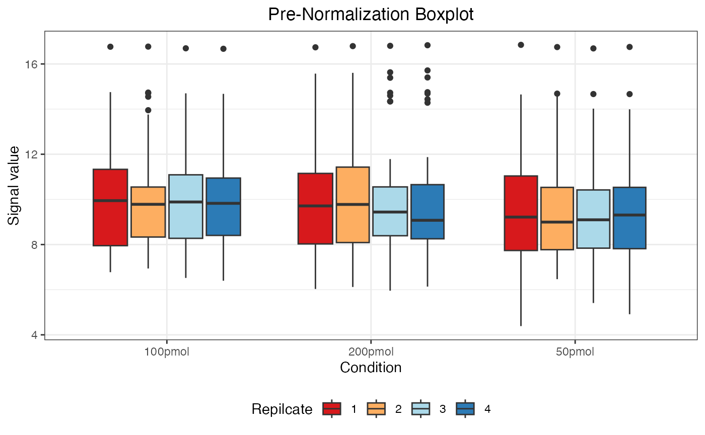
#> Warning: Removed 55 rows containing non-finite outside the scale range
#> (`stat_boxplot()`).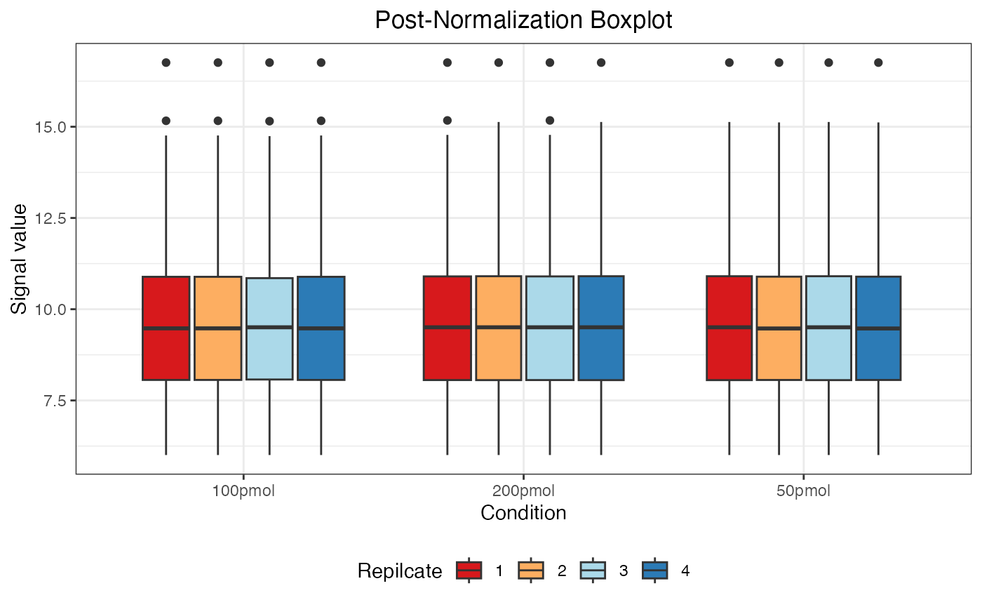
The message “Warning: Removed 55 rows containing non-finite values” indicates the presence of 55 NA (Not Available) values in the data. These NA values arise when a protein was not identified in a particular sample or condition and are automatically excluded when generating the boxplot but retained in the actual dataset.
| R.Condition | R.Replicate | NUD4B_HUMAN | A0A7P0T808_HUMAN | A0A8I5KU53_HUMAN | ZN840_HUMAN | CC85C_HUMAN | TMC5B_HUMAN | C9JEV0_HUMAN | C9JNU9_HUMAN | ALBU_BOVIN | CYC_BOVIN | TRFE_BOVIN | KRT16_MOUSE | F8W0H2_HUMAN | H0Y7V7_HUMAN | H0YD14_HUMAN | H3BUF6_HUMAN | H7C1W4_HUMAN | H7C3M7_HUMAN | TCPR2_HUMAN | TLR3_HUMAN | LRIG2_HUMAN | RAB3D_HUMAN | ADH1_YEAST | LYSC_CHICK | BGAL_ECOLI | CYTA_HUMAN | KPCB_HUMAN | LIPL_HUMAN | PIP_HUMAN | CO6_HUMAN | BGAL_HUMAN | SYTC_HUMAN | CASPE_HUMAN | DCAF6_HUMAN | DALD3_HUMAN | HGNAT_HUMAN | RFFL_HUMAN | RN185_HUMAN | ZN462_HUMAN | ALKB7_HUMAN | POLK_HUMAN | ACAD8_HUMAN | A0A7I2PK40_HUMAN | NBDY_HUMAN | H0Y5R1_HUMAN |
|---|---|---|---|---|---|---|---|---|---|---|---|---|---|---|---|---|---|---|---|---|---|---|---|---|---|---|---|---|---|---|---|---|---|---|---|---|---|---|---|---|---|---|---|---|---|---|
| 100pmol | 1 | 10.37045 | 11.406514 | 10.956950 | 8.392426 | 8.710518 | 8.610420 | 7.829510 | 8.023133 | 16.75777 | 12.96499 | 13.97388 | 10.51096 | 9.136271 | 10.231965 | 10.048461 | 8.179306 | 8.279169 | 9.874410 | 14.201118 | 7.001503 | 8.832972 | 9.978488 | 15.16303 | 13.62766 | 14.44005 | 8.964155 | 9.574185 | 8.517979 | 6.420716 | 6.764393 | 12.07953 | 14.76033 | 6.004586 | 7.670711 | 10.129049 | 10.681337 | 7.242036 | 9.727210 | 9.376507 | 7.109682 | 7.393910 | 7.530379 | NA | NA | NA |
| 100pmol | 2 | 11.40651 | 12.964987 | 9.727210 | 8.517979 | 8.832972 | 8.710518 | 7.242036 | 8.023133 | 16.75777 | 13.62766 | 14.20112 | NA | 8.964155 | 10.048461 | 10.231965 | 7.829510 | 7.670711 | 9.574185 | 10.681337 | 7.393910 | 8.610420 | 10.129049 | 15.16303 | 13.97388 | 14.44005 | 9.136271 | 9.978488 | 8.279169 | 6.764393 | 6.420716 | 12.07953 | 14.76033 | 7.109682 | 8.179306 | 9.874410 | 10.956950 | 7.001503 | 10.370449 | 8.392426 | 6.004586 | 9.376507 | 7.530379 | 10.510962 | NA | NA |
| 100pmol | 3 | 10.32522 | 11.893804 | 10.851852 | 7.868171 | 8.887142 | NA | 6.429596 | 8.646475 | 16.75777 | 12.81909 | 13.94448 | NA | 9.027184 | 9.940284 | 9.504539 | 8.074082 | 7.698334 | 10.467264 | 14.178809 | 7.413486 | 8.433160 | 10.022816 | 15.15272 | 13.55168 | 14.42169 | 8.758911 | 9.812352 | 8.213284 | NA | 6.777937 | 11.29130 | 14.74334 | 6.004586 | 8.311138 | 9.649565 | 10.097660 | 7.009435 | 10.195272 | 8.550204 | 7.121143 | 7.262869 | 7.555404 | 10.625304 | 9.244669 | NA |
| 100pmol | 4 | 10.51096 | 12.079525 | 10.956950 | 8.279169 | 8.964155 | 8.610420 | 6.004586 | 8.023133 | 16.75777 | 12.96499 | 13.97388 | NA | 9.136271 | 10.048461 | 9.978488 | NA | 7.670711 | 9.376507 | 14.440054 | 7.829510 | 8.517979 | 10.231965 | 15.16303 | 13.62766 | 14.20112 | 8.710518 | 10.129049 | 8.179306 | NA | 7.109682 | 11.40651 | 14.76033 | 6.420716 | 7.530379 | 8.832972 | 10.681337 | 6.764393 | 9.874410 | 8.392426 | 7.001503 | 7.242036 | 7.393910 | 10.370449 | 9.727210 | 9.574185 |
| 200pmol | 1 | 10.27762 | 12.256403 | 10.413259 | 8.356482 | 7.375266 | 8.476493 | 7.098768 | NA | 16.75777 | 13.10393 | 14.00189 | 10.74088 | 9.255807 | 10.077232 | 9.798890 | 8.142561 | 7.974610 | 10.164570 | 13.700017 | 7.644405 | 8.253204 | 9.927121 | 15.17286 | 14.22236 | 14.77650 | 8.577167 | 10.010298 | 8.782531 | 6.004586 | 7.222195 | 11.51625 | 14.45755 | 6.412260 | 7.506546 | 9.641587 | 10.556023 | 6.751494 | 8.669939 | 9.040857 | 7.792691 | 6.993948 | 8.905805 | 11.057043 | NA | 9.504539 |
| 200pmol | 2 | 10.53171 | 11.078642 | 10.729201 | NA | 8.732804 | NA | 7.026553 | 8.267212 | 16.75777 | 12.49496 | 13.38772 | NA | 9.012072 | 10.120238 | NA | 8.149770 | 7.964140 | 9.954832 | 14.130668 | 7.608925 | 8.620541 | 10.229206 | 15.13045 | 13.88102 | 14.70670 | 8.866513 | 10.377729 | 8.386314 | NA | 7.145874 | 11.59517 | 14.38206 | 6.004586 | 7.766206 | 9.827232 | 9.232358 | 6.448756 | 9.504539 | 8.520402 | 6.807164 | 7.455730 | 7.307825 | NA | 10.036651 | 9.658384 |
| 200pmol | 3 | 11.05704 | 8.142561 | 12.256403 | 8.356482 | 8.905805 | 8.782531 | 6.412260 | 8.669939 | 16.75777 | 14.00189 | 13.70002 | 10.74088 | 9.255807 | 10.413259 | 10.164570 | 7.792691 | 7.506546 | 10.010298 | NA | 7.375266 | 8.476493 | 10.277619 | 15.17286 | 14.22236 | 14.77650 | 8.577167 | 9.927121 | 8.253204 | NA | 6.993948 | 13.10393 | 14.45755 | 6.004586 | 7.098768 | 10.077232 | 11.516245 | 6.751494 | 9.798890 | 9.040857 | 7.974610 | 7.222195 | 7.644405 | 10.556023 | 9.641587 | 9.504539 |
| 200pmol | 4 | 10.72920 | 8.520402 | 11.595175 | 8.732804 | 7.964140 | 9.012072 | 6.448756 | 8.149770 | 16.75777 | 13.38772 | 13.88102 | NA | 9.504539 | 9.954832 | 10.229206 | 8.267212 | 6.807164 | 10.036651 | NA | 7.455730 | NA | 10.531713 | 15.13045 | 14.13067 | 14.70670 | 9.232358 | 10.377729 | 8.386314 | NA | 7.026553 | 12.49496 | 14.38206 | 6.004586 | 7.608925 | 10.120238 | 11.078642 | 7.145874 | 9.658384 | 8.866513 | 7.766206 | 7.307825 | 8.620541 | 9.827232 | NA | NA |
| 50pmol | 1 | 10.72920 | 9.232358 | 7.766206 | 8.267212 | 8.732804 | NA | 9.658384 | 7.964140 | 16.75777 | 12.49496 | 13.88102 | NA | 9.504539 | 10.120238 | 10.377729 | 8.520402 | 7.608925 | 9.827232 | 14.130668 | 7.455730 | 8.620541 | 10.531713 | 14.70670 | 13.38772 | 14.38206 | 11.078642 | 10.229206 | 8.386314 | 10.036651 | 7.026553 | 11.59517 | 15.13045 | 9.954832 | 7.307825 | NA | 9.012072 | 6.807164 | 8.866513 | 6.448756 | 8.149770 | 6.004586 | 7.145874 | NA | NA | NA |
| 50pmol | 2 | 10.96831 | NA | 10.662903 | 8.659793 | 8.785723 | NA | 8.190682 | 8.555305 | 16.75777 | 12.30540 | 13.84672 | NA | 9.753718 | 9.581714 | 10.189464 | 8.429646 | 7.035806 | 10.008606 | 14.686886 | 7.159242 | 9.099265 | 10.482590 | 14.36063 | 13.25790 | 14.10465 | 10.086066 | NA | 8.926299 | 7.806291 | 7.637117 | 11.47571 | 15.11842 | 8.017625 | 7.480137 | 8.298269 | 10.329078 | 6.459113 | 9.911682 | 9.362666 | 7.332126 | 6.004586 | 6.822962 | NA | NA | NA |
| 50pmol | 3 | 11.59517 | 6.004586 | 10.729201 | 6.448756 | 8.732804 | 9.232358 | 8.149770 | 8.386314 | 16.75777 | 13.38772 | 14.13067 | 11.07864 | 9.658384 | NA | 10.377729 | 8.620541 | 7.026553 | 9.954832 | 9.827232 | NA | NA | 10.531713 | 14.70670 | 13.88102 | 14.38206 | 10.036651 | 10.229206 | 9.012072 | 7.608925 | 7.455730 | 12.49496 | 15.13045 | 7.964140 | 7.766206 | 8.520402 | 10.120238 | 7.145874 | 9.504539 | 8.267212 | 8.866513 | 7.307825 | 6.807164 | NA | NA | NA |
| 50pmol | 4 | 10.96831 | 10.008606 | 10.662903 | 8.298269 | 8.190682 | 8.785723 | 7.806291 | 8.659793 | 16.75777 | 12.30540 | 13.84672 | NA | NA | 9.362666 | 10.482590 | 8.555305 | 6.004586 | 9.753718 | 14.360635 | 7.035806 | 8.429646 | 10.329078 | 14.68689 | 13.25790 | 14.10465 | 9.911682 | 10.189464 | NA | 7.332126 | NA | 11.47571 | 15.11842 | 7.637117 | 8.017625 | 9.581714 | 10.086066 | 6.459113 | 9.099265 | 8.926299 | 7.480137 | 7.159242 | 6.822962 | NA | NA | NA |
Imputation
Usage
dataMissing(
  dataSet,                # dataset of experimental values
  sort_miss = FALSE,      # should columns be ordered by missingness?
  plot = FALSE,           # should missingness be plotted?
  show_pct_legend = TRUE, # should % missing be displayed on plot?
  show_labels = TRUE,     # should column headings be displayed on plot?
  show_pct_col = TRUE     # should % missing by column be displayed on plot?
)

impute.min_local(dataSet,                  # dataset of experimental values
                 reportImputing = FALSE,   # should a record of imputed values be kept?
                 reqPercentPresent = 0.51) # what percent of replicates should be experimentally observed for the others to be imputed?

impute.min_global(dataSet,                # dataset of experimental values
                  reportImputing = FALSE) # should a record of imputed values be kept?

impute.knn_seq(dataSet,                # dataset of experimental values
               reportImputing = FALSE, # should a record of imputed values be kept?
               k = 10)                 # number of neighbors for imputation
Details & Examples
The two primary MS/MS acquisition types implemented in large scale MS-based proteomics have unique advantages and disadvantages. Traditional Data-Dependent Acquisition (DDA) methods favor specificity in MS/MS sampling over comprehensive proteome coverage. Small peptide isolation windows (<3 m/z) result in MS/MS spectra that contain fragmentation data from ideally only one peptide. This specificity promotes clear peptide identifications but comes at the expense of added scan time. In DDA experiments, the number of peptides that can be selected for MS/MS is limited by instrument scan speeds and is therefore prioritized by highest peptide abundance. Low abundance peptides are sampled less frequently for MS/MS and this can result in variable peptide coverage and many missing protein data across large sample datasets.
Data-Independent Acquisition (DIA) methods promote comprehensive peptide coverage over specificity by sampling many peptides for MS/MS simultaneously. Sequential and large mass isolation windows (4-50 m/z) are used to isolate large numbers of peptides at once for concurrent MS/MS. This produces complicated fragmentation spectra, but these spectra contain data on every observable peptide. A major disadvantage with this type of acquisition is that DIA MS/MS spectra are incredibly complex and difficult to deconvolve. Powerful and relatively new software programs like Spectronaut are capable of successfully parsing out which fragment ions came from each co-fragmented peptide using custom libraries, machine learning algorithms, and precisely determined retention times or measured ion mobility data. Because all observable ions are sampled for MS/MS, DIA reduces missingness substantially compared to DDA, though not entirely.
Function dataMissing() is designed to summarize the
missingness for each protein, where plot = TRUE indicates
plotting the missingness, and show_labels = TRUE means that
the protein names are displayed in the printed plot. Note that the
visual representation is not generated by default, and the plot
generation time varies with project size.
dataMissing <- dataMissing(dataNorm, plot = TRUE, show_labels = TRUE)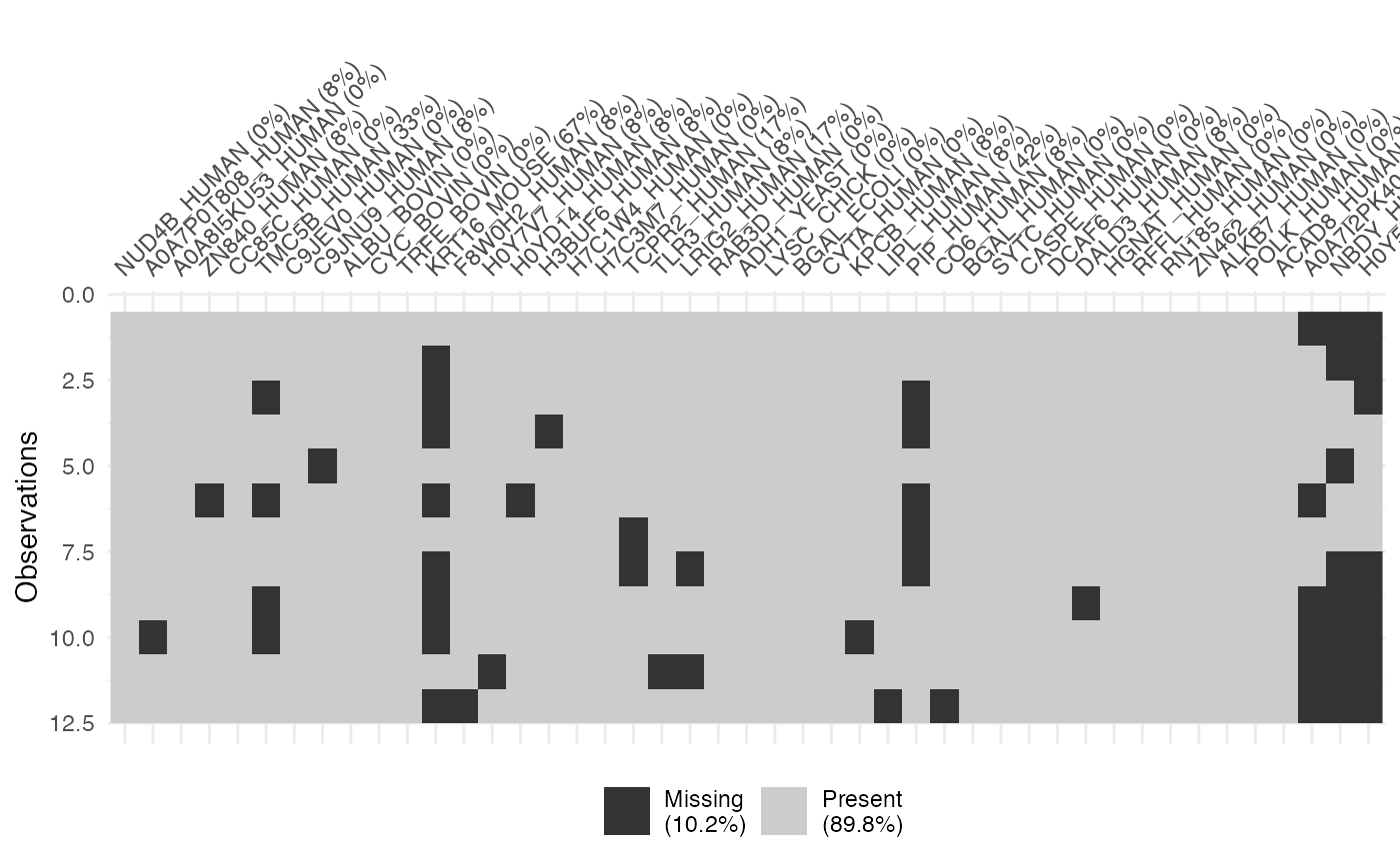
The percentage in the protein labels represents the proportion of
missing data in the samples for that protein. For instance, the label
“ZN840_HUMAN (8%)” indicates that, within all observations for the
protein “ZN840_HUMAN”, 8% of the data is missing. Additionally, the
percentage in the legend represents the proportion of missing data in
the whole dataset. In this case, 10.2% of the data in
dataNorm is missing.
Regardless of plot generation, the function
dataMissing() always returns a table providing the
following information:
count_miss: The count of missing values for each protein.pct_miss_col: The percentage of missing values for each protein.pct_miss_tot: The percentage of missing values for each protein relative to the total missing values in the entire dataset.
| NUD4B_HUMAN | A0A7P0T808_HUMAN | A0A8I5KU53_HUMAN | ZN840_HUMAN | CC85C_HUMAN | TMC5B_HUMAN | C9JEV0_HUMAN | C9JNU9_HUMAN | ALBU_BOVIN | CYC_BOVIN | TRFE_BOVIN | KRT16_MOUSE | F8W0H2_HUMAN | H0Y7V7_HUMAN | H0YD14_HUMAN | H3BUF6_HUMAN | H7C1W4_HUMAN | H7C3M7_HUMAN | TCPR2_HUMAN | TLR3_HUMAN | LRIG2_HUMAN | RAB3D_HUMAN | ADH1_YEAST | LYSC_CHICK | BGAL_ECOLI | CYTA_HUMAN | KPCB_HUMAN | LIPL_HUMAN | PIP_HUMAN | CO6_HUMAN | BGAL_HUMAN | SYTC_HUMAN | CASPE_HUMAN | DCAF6_HUMAN | DALD3_HUMAN | HGNAT_HUMAN | RFFL_HUMAN | RN185_HUMAN | ZN462_HUMAN | ALKB7_HUMAN | POLK_HUMAN | ACAD8_HUMAN | A0A7I2PK40_HUMAN | NBDY_HUMAN | H0Y5R1_HUMAN | |
|---|---|---|---|---|---|---|---|---|---|---|---|---|---|---|---|---|---|---|---|---|---|---|---|---|---|---|---|---|---|---|---|---|---|---|---|---|---|---|---|---|---|---|---|---|---|
| count_miss | 0 | 1.000000 | 0 | 1.000000 | 0 | 4.000000 | 0 | 1.000000 | 0 | 0 | 0 | 8.00000 | 1.000000 | 1.000000 | 1.000000 | 1.000000 | 0 | 0 | 2.000000 | 1.000000 | 2.000000 | 0 | 0 | 0 | 0 | 0 | 1.000000 | 1.000000 | 5.000000 | 1.000000 | 0 | 0 | 0 | 0 | 1.000000 | 0 | 0 | 0 | 0 | 0 | 0 | 0 | 6.00000 | 8.00000 | 8.00000 |
| pct_miss_col | 0 | 8.333333 | 0 | 8.333333 | 0 | 33.333333 | 0 | 8.333333 | 0 | 0 | 0 | 66.66667 | 8.333333 | 8.333333 | 8.333333 | 8.333333 | 0 | 0 | 16.666667 | 8.333333 | 16.666667 | 0 | 0 | 0 | 0 | 0 | 8.333333 | 8.333333 | 41.666667 | 8.333333 | 0 | 0 | 0 | 0 | 8.333333 | 0 | 0 | 0 | 0 | 0 | 0 | 0 | 50.00000 | 66.66667 | 66.66667 |
| pct_miss_tot | 0 | 1.818182 | 0 | 1.818182 | 0 | 7.272727 | 0 | 1.818182 | 0 | 0 | 0 | 14.54545 | 1.818182 | 1.818182 | 1.818182 | 1.818182 | 0 | 0 | 3.636364 | 1.818182 | 3.636364 | 0 | 0 | 0 | 0 | 0 | 1.818182 | 1.818182 | 9.090909 | 1.818182 | 0 | 0 | 0 | 0 | 1.818182 | 0 | 0 | 0 | 0 | 0 | 0 | 0 | 10.90909 | 14.54545 | 14.54545 |
For example, in the case of the protein “ZN840_HUMAN,” there are 1 NA values in the samples, representing 8.33% of the missing data for “ZN840_HUMAN” within that sample and 1.82% of the total missing data in the entire dataset.
Various imputation methods have been developed to address the missing-value issue and assign a reasonable guess of quantitative value to proteins with missing values. So far, this package provides 10 imputation methods for use:
impute.min_local(): Replaces missing values with the lowest measured value for that protein in that condition.impute.min_global(): Replaces missing values with the lowest measured value from any protein found within the entire dataset.impute.knn(): Replaces missing values using the k-nearest neighbors algorithm (Troyanskaya et al. 2001).impute.knn_seq(): Replaces missing values using the sequential k-nearest neighbors algorithm (Kim, Kim, and Yi 2004).impute.knn_trunc(): Replaces missing values using the truncated k-nearest neighbors algorithm (Shah et al. 2017).impute.nuc_norm(): Replaces missing values using the nuclear-norm regularization (Hastie et al. 2015).impute.mice_cart(): Replaces missing values using the classification and regression trees (Breiman et al. 1984; Doove, van Buuren, and Dusseldorp 2014; van Buuren 2018).impute.mice_norm(): Replaces missing values using the Bayesian linear regression (Rubin 1987; Schafer 1997; van Buuren and Groothuis-Oudshoorn 2011).impute.pca_bayes(): Replaces missing values using the Bayesian principal components analysis (Oba et al. 2003).impute.pca_prob(): Replaces missing values using the probabilistic principal components analysis (Stacklies et al. 2007).
Additional methods will be added later.
For example, to impute the NA value of dataNorm using
impute.min_local(), set the required percentage of values
that must be present in a given protein by condition combination for
values to be imputed to 51%.
reqPercentPresent to 0.51 requires that any
protein be observed in a majority of the replicates by condition in
order to be considered. For 3 replicates, this would require 2
measurements to allow imputation of the 3rd value. If only 1 measurement
is seen, the other values will remain NA, and will be filtered out in a
subsequent step.
dataImput <- impute.min_local(dataNorm, reportImputing = FALSE,
reqPercentPresent = 0.51)| R.Condition | R.Replicate | NUD4B_HUMAN | A0A7P0T808_HUMAN | A0A8I5KU53_HUMAN | ZN840_HUMAN | CC85C_HUMAN | TMC5B_HUMAN | C9JEV0_HUMAN | C9JNU9_HUMAN | ALBU_BOVIN | CYC_BOVIN | TRFE_BOVIN | KRT16_MOUSE | F8W0H2_HUMAN | H0Y7V7_HUMAN | H0YD14_HUMAN | H3BUF6_HUMAN | H7C1W4_HUMAN | H7C3M7_HUMAN | TCPR2_HUMAN | TLR3_HUMAN | LRIG2_HUMAN | RAB3D_HUMAN | ADH1_YEAST | LYSC_CHICK | BGAL_ECOLI | CYTA_HUMAN | KPCB_HUMAN | LIPL_HUMAN | PIP_HUMAN | CO6_HUMAN | BGAL_HUMAN | SYTC_HUMAN | CASPE_HUMAN | DCAF6_HUMAN | DALD3_HUMAN | HGNAT_HUMAN | RFFL_HUMAN | RN185_HUMAN | ZN462_HUMAN | ALKB7_HUMAN | POLK_HUMAN | ACAD8_HUMAN | A0A7I2PK40_HUMAN | NBDY_HUMAN | H0Y5R1_HUMAN |
|---|---|---|---|---|---|---|---|---|---|---|---|---|---|---|---|---|---|---|---|---|---|---|---|---|---|---|---|---|---|---|---|---|---|---|---|---|---|---|---|---|---|---|---|---|---|---|
| 100pmol | 1 | 10.37045 | 11.406514 | 10.956950 | 8.392426 | 8.710518 | 8.610420 | 7.829510 | 8.023133 | 16.75777 | 12.96499 | 13.97388 | 10.51096 | 9.136271 | 10.231965 | 10.048461 | 8.179306 | 8.279169 | 9.874410 | 14.201118 | 7.001503 | 8.832972 | 9.978488 | 15.16303 | 13.62766 | 14.44005 | 8.964155 | 9.574185 | 8.517979 | 6.420716 | 6.764393 | 12.07953 | 14.76033 | 6.004586 | 7.670711 | 10.129049 | 10.681337 | 7.242036 | 9.727210 | 9.376507 | 7.109682 | 7.393910 | 7.530379 | 10.370449 | NA | NA |
| 100pmol | 2 | 11.40651 | 12.964987 | 9.727210 | 8.517979 | 8.832972 | 8.710518 | 7.242036 | 8.023133 | 16.75777 | 13.62766 | 14.20112 | NA | 8.964155 | 10.048461 | 10.231965 | 7.829510 | 7.670711 | 9.574185 | 10.681337 | 7.393910 | 8.610420 | 10.129049 | 15.16303 | 13.97388 | 14.44005 | 9.136271 | 9.978488 | 8.279169 | 6.764393 | 6.420716 | 12.07953 | 14.76033 | 7.109682 | 8.179306 | 9.874410 | 10.956950 | 7.001503 | 10.370449 | 8.392426 | 6.004586 | 9.376507 | 7.530379 | 10.510962 | NA | NA |
| 100pmol | 3 | 10.32522 | 11.893804 | 10.851852 | 7.868171 | 8.887142 | 8.610420 | 6.429596 | 8.646475 | 16.75777 | 12.81909 | 13.94448 | NA | 9.027184 | 9.940284 | 9.504539 | 8.074082 | 7.698334 | 10.467264 | 14.178809 | 7.413486 | 8.433160 | 10.022816 | 15.15272 | 13.55168 | 14.42169 | 8.758911 | 9.812352 | 8.213284 | NA | 6.777937 | 11.29130 | 14.74334 | 6.004586 | 8.311138 | 9.649565 | 10.097660 | 7.009435 | 10.195272 | 8.550204 | 7.121143 | 7.262869 | 7.555404 | 10.625304 | 9.244669 | NA |
| 100pmol | 4 | 10.51096 | 12.079525 | 10.956950 | 8.279169 | 8.964155 | 8.610420 | 6.004586 | 8.023133 | 16.75777 | 12.96499 | 13.97388 | NA | 9.136271 | 10.048461 | 9.978488 | 7.829510 | 7.670711 | 9.376507 | 14.440054 | 7.829510 | 8.517979 | 10.231965 | 15.16303 | 13.62766 | 14.20112 | 8.710518 | 10.129049 | 8.179306 | NA | 7.109682 | 11.40651 | 14.76033 | 6.420716 | 7.530379 | 8.832972 | 10.681337 | 6.764393 | 9.874410 | 8.392426 | 7.001503 | 7.242036 | 7.393910 | 10.370449 | 9.727210 | 9.574185 |
| 200pmol | 1 | 10.27762 | 12.256403 | 10.413259 | 8.356482 | 7.375266 | 8.476493 | 7.098768 | 8.149770 | 16.75777 | 13.10393 | 14.00189 | 10.74088 | 9.255807 | 10.077232 | 9.798890 | 8.142561 | 7.974610 | 10.164570 | 13.700017 | 7.644405 | 8.253204 | 9.927121 | 15.17286 | 14.22236 | 14.77650 | 8.577167 | 10.010298 | 8.782531 | 6.004586 | 7.222195 | 11.51625 | 14.45755 | 6.412260 | 7.506546 | 9.641587 | 10.556023 | 6.751494 | 8.669939 | 9.040857 | 7.792691 | 6.993948 | 8.905805 | 11.057043 | NA | 9.504539 |
| 200pmol | 2 | 10.53171 | 11.078642 | 10.729201 | 8.356482 | 8.732804 | 8.476493 | 7.026553 | 8.267212 | 16.75777 | 12.49496 | 13.38772 | NA | 9.012072 | 10.120238 | 9.798890 | 8.149770 | 7.964140 | 9.954832 | 14.130668 | 7.608925 | 8.620541 | 10.229206 | 15.13045 | 13.88102 | 14.70670 | 8.866513 | 10.377729 | 8.386314 | NA | 7.145874 | 11.59517 | 14.38206 | 6.004586 | 7.766206 | 9.827232 | 9.232358 | 6.448756 | 9.504539 | 8.520402 | 6.807164 | 7.455730 | 7.307825 | 9.827232 | 10.036651 | 9.658384 |
| 200pmol | 3 | 11.05704 | 8.142561 | 12.256403 | 8.356482 | 8.905805 | 8.782531 | 6.412260 | 8.669939 | 16.75777 | 14.00189 | 13.70002 | 10.74088 | 9.255807 | 10.413259 | 10.164570 | 7.792691 | 7.506546 | 10.010298 | NA | 7.375266 | 8.476493 | 10.277619 | 15.17286 | 14.22236 | 14.77650 | 8.577167 | 9.927121 | 8.253204 | NA | 6.993948 | 13.10393 | 14.45755 | 6.004586 | 7.098768 | 10.077232 | 11.516245 | 6.751494 | 9.798890 | 9.040857 | 7.974610 | 7.222195 | 7.644405 | 10.556023 | 9.641587 | 9.504539 |
| 200pmol | 4 | 10.72920 | 8.520402 | 11.595175 | 8.732804 | 7.964140 | 9.012072 | 6.448756 | 8.149770 | 16.75777 | 13.38772 | 13.88102 | NA | 9.504539 | 9.954832 | 10.229206 | 8.267212 | 6.807164 | 10.036651 | NA | 7.455730 | 8.253204 | 10.531713 | 15.13045 | 14.13067 | 14.70670 | 9.232358 | 10.377729 | 8.386314 | NA | 7.026553 | 12.49496 | 14.38206 | 6.004586 | 7.608925 | 10.120238 | 11.078642 | 7.145874 | 9.658384 | 8.866513 | 7.766206 | 7.307825 | 8.620541 | 9.827232 | NA | 9.504539 |
| 50pmol | 1 | 10.72920 | 9.232358 | 7.766206 | 8.267212 | 8.732804 | NA | 9.658384 | 7.964140 | 16.75777 | 12.49496 | 13.88102 | NA | 9.504539 | 10.120238 | 10.377729 | 8.520402 | 7.608925 | 9.827232 | 14.130668 | 7.455730 | 8.620541 | 10.531713 | 14.70670 | 13.38772 | 14.38206 | 11.078642 | 10.229206 | 8.386314 | 10.036651 | 7.026553 | 11.59517 | 15.13045 | 9.954832 | 7.307825 | 8.298269 | 9.012072 | 6.807164 | 8.866513 | 6.448756 | 8.149770 | 6.004586 | 7.145874 | NA | NA | NA |
| 50pmol | 2 | 10.96831 | 6.004586 | 10.662903 | 8.659793 | 8.785723 | NA | 8.190682 | 8.555305 | 16.75777 | 12.30540 | 13.84672 | NA | 9.753718 | 9.581714 | 10.189464 | 8.429646 | 7.035806 | 10.008606 | 14.686886 | 7.159242 | 9.099265 | 10.482590 | 14.36063 | 13.25790 | 14.10465 | 10.086066 | 10.189464 | 8.926299 | 7.806291 | 7.637117 | 11.47571 | 15.11842 | 8.017625 | 7.480137 | 8.298269 | 10.329078 | 6.459113 | 9.911682 | 9.362666 | 7.332126 | 6.004586 | 6.822962 | NA | NA | NA |
| 50pmol | 3 | 11.59517 | 6.004586 | 10.729201 | 6.448756 | 8.732804 | 9.232358 | 8.149770 | 8.386314 | 16.75777 | 13.38772 | 14.13067 | 11.07864 | 9.658384 | 9.362666 | 10.377729 | 8.620541 | 7.026553 | 9.954832 | 9.827232 | 7.035806 | 8.429646 | 10.531713 | 14.70670 | 13.88102 | 14.38206 | 10.036651 | 10.229206 | 9.012072 | 7.608925 | 7.455730 | 12.49496 | 15.13045 | 7.964140 | 7.766206 | 8.520402 | 10.120238 | 7.145874 | 9.504539 | 8.267212 | 8.866513 | 7.307825 | 6.807164 | NA | NA | NA |
| 50pmol | 4 | 10.96831 | 10.008606 | 10.662903 | 8.298269 | 8.190682 | 8.785723 | 7.806291 | 8.659793 | 16.75777 | 12.30540 | 13.84672 | NA | 9.504539 | 9.362666 | 10.482590 | 8.555305 | 6.004586 | 9.753718 | 14.360635 | 7.035806 | 8.429646 | 10.329078 | 14.68689 | 13.25790 | 14.10465 | 9.911682 | 10.189464 | 8.386314 | 7.332126 | 7.026553 | 11.47571 | 15.11842 | 7.637117 | 8.017625 | 9.581714 | 10.086066 | 6.459113 | 9.099265 | 8.926299 | 7.480137 | 7.159242 | 6.822962 | NA | NA | NA |
If reportImputing = TRUE, the returned result structure
will be altered to a list, adding a shadow data frame with imputed data
labels, where 1 indicates the corresponding entries have been imputed,
and 0 indicates otherwise.
After the above imputation, any entries that did not pass the percent present threshold will still have NA values and will need to be filtered out.
dataImput <- filterNA(dataImput, saveRm = TRUE)where saveRm = TRUE indicates that the filtered data
will be saved as a .csv file named filtered_NA_data.csv in the
current working directory.
The dataImput is as follows:
| R.Condition | R.Replicate | NUD4B_HUMAN | A0A7P0T808_HUMAN | A0A8I5KU53_HUMAN | ZN840_HUMAN | CC85C_HUMAN | C9JEV0_HUMAN | C9JNU9_HUMAN | ALBU_BOVIN | CYC_BOVIN | TRFE_BOVIN | F8W0H2_HUMAN | H0Y7V7_HUMAN | H0YD14_HUMAN | H3BUF6_HUMAN | H7C1W4_HUMAN | H7C3M7_HUMAN | TLR3_HUMAN | LRIG2_HUMAN | RAB3D_HUMAN | ADH1_YEAST | LYSC_CHICK | BGAL_ECOLI | CYTA_HUMAN | KPCB_HUMAN | LIPL_HUMAN | CO6_HUMAN | BGAL_HUMAN | SYTC_HUMAN | CASPE_HUMAN | DCAF6_HUMAN | DALD3_HUMAN | HGNAT_HUMAN | RFFL_HUMAN | RN185_HUMAN | ZN462_HUMAN | ALKB7_HUMAN | POLK_HUMAN | ACAD8_HUMAN |
|---|---|---|---|---|---|---|---|---|---|---|---|---|---|---|---|---|---|---|---|---|---|---|---|---|---|---|---|---|---|---|---|---|---|---|---|---|---|---|---|
| 100pmol | 1 | 10.37045 | 11.406514 | 10.956950 | 8.392426 | 8.710518 | 7.829510 | 8.023133 | 16.75777 | 12.96499 | 13.97388 | 9.136271 | 10.231965 | 10.048461 | 8.179306 | 8.279169 | 9.874410 | 7.001503 | 8.832972 | 9.978488 | 15.16303 | 13.62766 | 14.44005 | 8.964155 | 9.574185 | 8.517979 | 6.764393 | 12.07953 | 14.76033 | 6.004586 | 7.670711 | 10.129049 | 10.681337 | 7.242036 | 9.727210 | 9.376507 | 7.109682 | 7.393910 | 7.530379 |
| 100pmol | 2 | 11.40651 | 12.964987 | 9.727210 | 8.517979 | 8.832972 | 7.242036 | 8.023133 | 16.75777 | 13.62766 | 14.20112 | 8.964155 | 10.048461 | 10.231965 | 7.829510 | 7.670711 | 9.574185 | 7.393910 | 8.610420 | 10.129049 | 15.16303 | 13.97388 | 14.44005 | 9.136271 | 9.978488 | 8.279169 | 6.420716 | 12.07953 | 14.76033 | 7.109682 | 8.179306 | 9.874410 | 10.956950 | 7.001503 | 10.370449 | 8.392426 | 6.004586 | 9.376507 | 7.530379 |
| 100pmol | 3 | 10.32522 | 11.893804 | 10.851852 | 7.868171 | 8.887142 | 6.429596 | 8.646475 | 16.75777 | 12.81909 | 13.94448 | 9.027184 | 9.940284 | 9.504539 | 8.074082 | 7.698334 | 10.467264 | 7.413486 | 8.433160 | 10.022816 | 15.15272 | 13.55168 | 14.42169 | 8.758911 | 9.812352 | 8.213284 | 6.777937 | 11.29130 | 14.74334 | 6.004586 | 8.311138 | 9.649565 | 10.097660 | 7.009435 | 10.195272 | 8.550204 | 7.121143 | 7.262869 | 7.555404 |
| 100pmol | 4 | 10.51096 | 12.079525 | 10.956950 | 8.279169 | 8.964155 | 6.004586 | 8.023133 | 16.75777 | 12.96499 | 13.97388 | 9.136271 | 10.048461 | 9.978488 | 7.829510 | 7.670711 | 9.376507 | 7.829510 | 8.517979 | 10.231965 | 15.16303 | 13.62766 | 14.20112 | 8.710518 | 10.129049 | 8.179306 | 7.109682 | 11.40651 | 14.76033 | 6.420716 | 7.530379 | 8.832972 | 10.681337 | 6.764393 | 9.874410 | 8.392426 | 7.001503 | 7.242036 | 7.393910 |
| 200pmol | 1 | 10.27762 | 12.256403 | 10.413259 | 8.356482 | 7.375266 | 7.098768 | 8.149770 | 16.75777 | 13.10393 | 14.00189 | 9.255807 | 10.077232 | 9.798890 | 8.142561 | 7.974610 | 10.164570 | 7.644405 | 8.253204 | 9.927121 | 15.17286 | 14.22236 | 14.77650 | 8.577167 | 10.010298 | 8.782531 | 7.222195 | 11.51625 | 14.45755 | 6.412260 | 7.506546 | 9.641587 | 10.556023 | 6.751494 | 8.669939 | 9.040857 | 7.792691 | 6.993948 | 8.905805 |
| 200pmol | 2 | 10.53171 | 11.078642 | 10.729201 | 8.356482 | 8.732804 | 7.026553 | 8.267212 | 16.75777 | 12.49496 | 13.38772 | 9.012072 | 10.120238 | 9.798890 | 8.149770 | 7.964140 | 9.954832 | 7.608925 | 8.620541 | 10.229206 | 15.13045 | 13.88102 | 14.70670 | 8.866513 | 10.377729 | 8.386314 | 7.145874 | 11.59517 | 14.38206 | 6.004586 | 7.766206 | 9.827232 | 9.232358 | 6.448756 | 9.504539 | 8.520402 | 6.807164 | 7.455730 | 7.307825 |
| 200pmol | 3 | 11.05704 | 8.142561 | 12.256403 | 8.356482 | 8.905805 | 6.412260 | 8.669939 | 16.75777 | 14.00189 | 13.70002 | 9.255807 | 10.413259 | 10.164570 | 7.792691 | 7.506546 | 10.010298 | 7.375266 | 8.476493 | 10.277619 | 15.17286 | 14.22236 | 14.77650 | 8.577167 | 9.927121 | 8.253204 | 6.993948 | 13.10393 | 14.45755 | 6.004586 | 7.098768 | 10.077232 | 11.516245 | 6.751494 | 9.798890 | 9.040857 | 7.974610 | 7.222195 | 7.644405 |
| 200pmol | 4 | 10.72920 | 8.520402 | 11.595175 | 8.732804 | 7.964140 | 6.448756 | 8.149770 | 16.75777 | 13.38772 | 13.88102 | 9.504539 | 9.954832 | 10.229206 | 8.267212 | 6.807164 | 10.036651 | 7.455730 | 8.253204 | 10.531713 | 15.13045 | 14.13067 | 14.70670 | 9.232358 | 10.377729 | 8.386314 | 7.026553 | 12.49496 | 14.38206 | 6.004586 | 7.608925 | 10.120238 | 11.078642 | 7.145874 | 9.658384 | 8.866513 | 7.766206 | 7.307825 | 8.620541 |
| 50pmol | 1 | 10.72920 | 9.232358 | 7.766206 | 8.267212 | 8.732804 | 9.658384 | 7.964140 | 16.75777 | 12.49496 | 13.88102 | 9.504539 | 10.120238 | 10.377729 | 8.520402 | 7.608925 | 9.827232 | 7.455730 | 8.620541 | 10.531713 | 14.70670 | 13.38772 | 14.38206 | 11.078642 | 10.229206 | 8.386314 | 7.026553 | 11.59517 | 15.13045 | 9.954832 | 7.307825 | 8.298269 | 9.012072 | 6.807164 | 8.866513 | 6.448756 | 8.149770 | 6.004586 | 7.145874 |
| 50pmol | 2 | 10.96831 | 6.004586 | 10.662903 | 8.659793 | 8.785723 | 8.190682 | 8.555305 | 16.75777 | 12.30540 | 13.84672 | 9.753718 | 9.581714 | 10.189464 | 8.429646 | 7.035806 | 10.008606 | 7.159242 | 9.099265 | 10.482590 | 14.36063 | 13.25790 | 14.10465 | 10.086066 | 10.189464 | 8.926299 | 7.637117 | 11.47571 | 15.11842 | 8.017625 | 7.480137 | 8.298269 | 10.329078 | 6.459113 | 9.911682 | 9.362666 | 7.332126 | 6.004586 | 6.822962 |
| 50pmol | 3 | 11.59517 | 6.004586 | 10.729201 | 6.448756 | 8.732804 | 8.149770 | 8.386314 | 16.75777 | 13.38772 | 14.13067 | 9.658384 | 9.362666 | 10.377729 | 8.620541 | 7.026553 | 9.954832 | 7.035806 | 8.429646 | 10.531713 | 14.70670 | 13.88102 | 14.38206 | 10.036651 | 10.229206 | 9.012072 | 7.455730 | 12.49496 | 15.13045 | 7.964140 | 7.766206 | 8.520402 | 10.120238 | 7.145874 | 9.504539 | 8.267212 | 8.866513 | 7.307825 | 6.807164 |
| 50pmol | 4 | 10.96831 | 10.008606 | 10.662903 | 8.298269 | 8.190682 | 7.806291 | 8.659793 | 16.75777 | 12.30540 | 13.84672 | 9.504539 | 9.362666 | 10.482590 | 8.555305 | 6.004586 | 9.753718 | 7.035806 | 8.429646 | 10.329078 | 14.68689 | 13.25790 | 14.10465 | 9.911682 | 10.189464 | 8.386314 | 7.026553 | 11.47571 | 15.11842 | 7.637117 | 8.017625 | 9.581714 | 10.086066 | 6.459113 | 9.099265 | 8.926299 | 7.480137 | 7.159242 | 6.822962 |
Summarization
Usage
summarize(dataSet,         # dataset of experimental values
          saveSumm = TRUE) # save a table of summary statistics?
Details & Examples
This summarization provides a table of values for each protein in the final dataset that include the final processed abundances and fold changes in each condition, and that protein’s statistical relation to the global dataset in terms of its mean, median, standard deviation, and other parameters.
dataSumm <- summarize(dataImput, saveSumm = TRUE)| Condition | Stat | NUD4B_HUMAN | A0A7P0T808_HUMAN | A0A8I5KU53_HUMAN | ZN840_HUMAN | CC85C_HUMAN | C9JEV0_HUMAN | C9JNU9_HUMAN | ALBU_BOVIN | CYC_BOVIN | TRFE_BOVIN | F8W0H2_HUMAN | H0Y7V7_HUMAN | H0YD14_HUMAN | H3BUF6_HUMAN | H7C1W4_HUMAN | H7C3M7_HUMAN | TLR3_HUMAN | LRIG2_HUMAN | RAB3D_HUMAN | ADH1_YEAST | LYSC_CHICK | BGAL_ECOLI | CYTA_HUMAN | KPCB_HUMAN | LIPL_HUMAN | CO6_HUMAN | BGAL_HUMAN | SYTC_HUMAN | CASPE_HUMAN | DCAF6_HUMAN | DALD3_HUMAN | HGNAT_HUMAN | RFFL_HUMAN | RN185_HUMAN | ZN462_HUMAN | ALKB7_HUMAN | POLK_HUMAN | ACAD8_HUMAN |
|---|---|---|---|---|---|---|---|---|---|---|---|---|---|---|---|---|---|---|---|---|---|---|---|---|---|---|---|---|---|---|---|---|---|---|---|---|---|---|---|
| 100pmol | n | 4.0000000 | 4.0000000 | 4.0000000 | 4.0000000 | 4.0000000 | 4.0000000 | 4.0000000 | 4.00000 | 4.0000000 | 4.0000000 | 4.0000000 | 4.0000000 | 4.0000000 | 4.0000000 | 4.0000000 | 4.0000000 | 4.0000000 | 4.0000000 | 4.0000000 | 4.0000000 | 4.0000000 | 4.0000000 | 4.0000000 | 4.0000000 | 4.0000000 | 4.0000000 | 4.0000000 | 4.0000000 | 4.0000000 | 4.0000000 | 4.0000000 | 4.0000000 | 4.0000000 | 4.0000000 | 4.0000000 | 4.0000000 | 4.0000000 | 4.0000000 |
| 100pmol | mean | 10.6532858 | 12.0862074 | 10.6232407 | 8.2644365 | 8.8486965 | 6.8764321 | 8.1789684 | 16.75777 | 13.0941802 | 14.0233390 | 9.0659703 | 10.0672927 | 9.9408634 | 7.9781022 | 7.8297313 | 9.8230915 | 7.4096023 | 8.5986327 | 10.0905795 | 15.1604531 | 13.6952175 | 14.3757288 | 8.8924636 | 9.8735187 | 8.2974346 | 6.7681823 | 11.7142153 | 14.7560796 | 6.3848929 | 7.9228836 | 9.6214990 | 10.6043210 | 7.0043419 | 10.0418355 | 8.6778910 | 6.8092287 | 7.8188307 | 7.5025180 |
| 100pmol | sd | 0.5083417 | 0.6509735 | 0.5994044 | 0.2816079 | 0.1066916 | 0.8168644 | 0.3116711 | 0.00000 | 0.3622393 | 0.1193272 | 0.0851570 | 0.1210474 | 0.3098987 | 0.1768750 | 0.2999079 | 0.4757395 | 0.3381959 | 0.1721820 | 0.1134697 | 0.0051583 | 0.1891971 | 0.1167288 | 0.1962332 | 0.2378070 | 0.1527627 | 0.2813447 | 0.4244383 | 0.0084914 | 0.5214944 | 0.3804140 | 0.5609915 | 0.3619004 | 0.1950282 | 0.2935700 | 0.4716454 | 0.5391294 | 1.0406244 | 0.0733600 |
| 100pmol | median | 10.4407055 | 11.9866645 | 10.9044011 | 8.3357977 | 8.8600566 | 6.8358159 | 8.0231329 | 16.75777 | 12.9649865 | 13.9738814 | 9.0817277 | 10.0484610 | 10.0134747 | 7.9517960 | 7.6845225 | 9.7242975 | 7.4036982 | 8.5641998 | 10.0759323 | 15.1630323 | 13.6276559 | 14.4308715 | 8.8615327 | 9.8954204 | 8.2462263 | 6.7711653 | 11.7430198 | 14.7603253 | 6.2126514 | 7.9250089 | 9.7619876 | 10.6813371 | 7.0054690 | 10.0348410 | 8.4713152 | 7.0555925 | 7.3283898 | 7.5303791 |
| 100pmol | trimmed | 10.6532858 | 12.0862074 | 10.6232407 | 8.2644365 | 8.8486965 | 6.8764321 | 8.1789684 | 16.75777 | 13.0941802 | 14.0233390 | 9.0659703 | 10.0672927 | 9.9408634 | 7.9781022 | 7.8297313 | 9.8230915 | 7.4096023 | 8.5986327 | 10.0905795 | 15.1604531 | 13.6952175 | 14.3757288 | 8.8924636 | 9.8735187 | 8.2974346 | 6.7681823 | 11.7142153 | 14.7560796 | 6.3848929 | 7.9228836 | 9.6214990 | 10.6043210 | 7.0043419 | 10.0418355 | 8.6778910 | 6.8092287 | 7.8188307 | 7.5025180 |
| 100pmol | mad | 0.1376914 | 0.4989033 | 0.0779088 | 0.1770303 | 0.0972461 | 0.9173216 | 0.0000000 | 0.00000 | 0.1081516 | 0.0217987 | 0.0808661 | 0.0801917 | 0.1879022 | 0.1813007 | 0.0204763 | 0.3690956 | 0.3054035 | 0.1314032 | 0.1116108 | 0.0000000 | 0.0563232 | 0.0136146 | 0.1880212 | 0.2347672 | 0.0740280 | 0.2559629 | 0.4989033 | 0.0000000 | 0.3084771 | 0.4747480 | 0.3554415 | 0.2043118 | 0.1783076 | 0.3469740 | 0.1169605 | 0.0886895 | 0.1125840 | 0.0185508 |
| 100pmol | min | 10.3252183 | 11.4065141 | 9.7272105 | 7.8681709 | 8.7105178 | 6.0045864 | 8.0231329 | 16.75777 | 12.8190919 | 13.9444754 | 8.9641549 | 9.9402840 | 9.5045393 | 7.8295103 | 7.6707114 | 9.3765069 | 7.0015026 | 8.4331596 | 9.9784883 | 15.1527157 | 13.5516770 | 14.2011179 | 8.7105178 | 9.5741849 | 8.1793065 | 6.4207163 | 11.2912962 | 14.7433424 | 6.0045864 | 7.5303791 | 8.8329716 | 10.0976598 | 6.7643932 | 9.7272105 | 8.3924265 | 6.0045864 | 7.2420363 | 7.3939101 |
| 100pmol | max | 11.4065141 | 12.9649865 | 10.9569499 | 8.5179795 | 8.9641549 | 7.8295103 | 8.6464751 | 16.75777 | 13.6276559 | 14.2011179 | 9.1362711 | 10.2319649 | 10.2319649 | 8.1793065 | 8.2791689 | 10.4672641 | 7.8295103 | 8.8329716 | 10.2319649 | 15.1630323 | 13.9738814 | 14.4400544 | 9.1362711 | 10.1290492 | 8.5179795 | 7.1096825 | 12.0795254 | 14.7603253 | 7.1096825 | 8.3111376 | 10.1290492 | 10.9569499 | 7.2420363 | 10.3704495 | 9.3765069 | 7.1211431 | 9.3765069 | 7.5554037 |
| 100pmol | range | 1.0812958 | 1.5584724 | 1.2297394 | 0.6498087 | 0.2536371 | 1.8249239 | 0.6233422 | 0.00000 | 0.8085640 | 0.2566425 | 0.1721162 | 0.2916809 | 0.7274256 | 0.3497962 | 0.6084576 | 1.0907573 | 0.8280077 | 0.3998121 | 0.2534766 | 0.0103166 | 0.4222044 | 0.2389365 | 0.4257533 | 0.5548643 | 0.3386730 | 0.6889662 | 0.7882292 | 0.0169829 | 1.1050961 | 0.7807586 | 1.2960775 | 0.8592901 | 0.4776431 | 0.6432390 | 0.9840804 | 1.1165567 | 2.1344706 | 0.1614936 |
| 100pmol | skew | 0.6975575 | 0.3239948 | -0.7349674 | -0.4906058 | -0.2153643 | 0.0746172 | 0.7500000 | NaN | 0.6663690 | 0.7189584 | -0.1695960 | 0.3387430 | -0.4796405 | 0.1114972 | 0.7458050 | 0.3783514 | 0.0392202 | 0.3827303 | 0.1991275 | -0.7500000 | 0.6668586 | -0.7378644 | 0.2135796 | -0.1711657 | 0.5944647 | -0.0238336 | -0.0237842 | -0.7500000 | 0.4773224 | -0.0050802 | -0.4861771 | -0.4499095 | -0.0129955 | 0.0322210 | 0.6966507 | -0.7281063 | 0.7407580 | -0.6901803 |
| 100pmol | kurtosis | -1.7260359 | -1.8707238 | -1.6982833 | -1.8448761 | -1.9494341 | -2.1798795 | -1.6875000 | NaN | -1.7327385 | -1.7058522 | -2.2461322 | -1.8404530 | -1.8192490 | -2.3106519 | -1.6904097 | -1.9467364 | -1.8757984 | -1.9169430 | -2.1242147 | -1.6875000 | -1.7325055 | -1.6961436 | -2.1614305 | -2.0285590 | -1.8014680 | -1.8757000 | -2.4101207 | -1.6875000 | -1.9257747 | -2.3455313 | -1.8463172 | -1.8132208 | -1.8755701 | -2.2325877 | -1.7280983 | -1.7033814 | -1.6940017 | -1.7210573 |
| 100pmol | se | 0.2541708 | 0.3254868 | 0.2997022 | 0.1408039 | 0.0533458 | 0.4084322 | 0.1558356 | 0.00000 | 0.1811196 | 0.0596636 | 0.0425785 | 0.0605237 | 0.1549494 | 0.0884375 | 0.1499539 | 0.2378698 | 0.1690980 | 0.0860910 | 0.0567349 | 0.0025791 | 0.0945985 | 0.0583644 | 0.0981166 | 0.1189035 | 0.0763814 | 0.1406723 | 0.2122191 | 0.0042457 | 0.2607472 | 0.1902070 | 0.2804957 | 0.1809502 | 0.0975141 | 0.1467850 | 0.2358227 | 0.2695647 | 0.5203122 | 0.0366800 |
| 200pmol | n | 4.0000000 | 4.0000000 | 4.0000000 | 4.0000000 | 4.0000000 | 4.0000000 | 4.0000000 | 4.00000 | 4.0000000 | 4.0000000 | 4.0000000 | 4.0000000 | 4.0000000 | 4.0000000 | 4.0000000 | 4.0000000 | 4.0000000 | 4.0000000 | 4.0000000 | 4.0000000 | 4.0000000 | 4.0000000 | 4.0000000 | 4.0000000 | 4.0000000 | 4.0000000 | 4.0000000 | 4.0000000 | 4.0000000 | 4.0000000 | 4.0000000 | 4.0000000 | 4.0000000 | 4.0000000 | 4.0000000 | 4.0000000 | 4.0000000 | 4.0000000 |
| 200pmol | mean | 10.6488941 | 9.9995022 | 11.2485095 | 8.4505628 | 8.2445037 | 6.7465842 | 8.3091726 | 16.75777 | 13.2471248 | 13.7426617 | 9.2570565 | 10.1413903 | 9.9978891 | 8.0880583 | 7.5631150 | 10.0415877 | 7.5210813 | 8.4008606 | 10.2414149 | 15.1516556 | 14.1141044 | 14.7415973 | 8.8133014 | 10.1732192 | 8.4520910 | 7.0971425 | 12.1775775 | 14.4198014 | 6.1065048 | 7.4951113 | 9.9165721 | 10.5958169 | 6.7744045 | 9.4079382 | 8.8671576 | 7.5851679 | 7.2449244 | 8.1196440 |
| 200pmol | sd | 0.3289432 | 1.9911564 | 0.8373275 | 0.1881608 | 0.7094445 | 0.3664652 | 0.2468009 | 0.00000 | 0.6260180 | 0.2671713 | 0.2010541 | 0.1943193 | 0.2312942 | 0.2050339 | 0.5491845 | 0.0887966 | 0.1270932 | 0.1803556 | 0.2480010 | 0.0244819 | 0.1612898 | 0.0403015 | 0.3108902 | 0.2385763 | 0.2290557 | 0.1059008 | 0.7605739 | 0.0435834 | 0.2038367 | 0.2849943 | 0.2242693 | 0.9901032 | 0.2858241 | 0.5064716 | 0.2453451 | 0.5268763 | 0.1931332 | 0.7646020 |
| 200pmol | median | 10.6304571 | 9.7995222 | 11.1621879 | 8.3564824 | 8.3484718 | 6.7376547 | 8.2084906 | 16.75777 | 13.2458280 | 13.7905186 | 9.2558074 | 10.0987350 | 9.9817300 | 8.1461655 | 7.7353428 | 10.0234743 | 7.5323272 | 8.3648486 | 10.2534127 | 15.1516556 | 14.1765162 | 14.7415973 | 8.7218404 | 10.1940134 | 8.3863145 | 7.0862137 | 12.0450654 | 14.4198014 | 6.0045864 | 7.5577355 | 9.9522318 | 10.8173322 | 6.7514941 | 9.5814615 | 8.9536853 | 7.7794486 | 7.2650103 | 8.1324727 |
| 200pmol | trimmed | 10.6488941 | 9.9995022 | 11.2485095 | 8.4505628 | 8.2445037 | 6.7465842 | 8.3091726 | 16.75777 | 13.2471248 | 13.7426617 | 9.2570565 | 10.1413903 | 9.9978891 | 8.0880583 | 7.5631150 | 10.0415877 | 7.5210813 | 8.4008606 | 10.2414149 | 15.1516556 | 14.1141044 | 14.7415973 | 8.8133014 | 10.1732192 | 8.4520910 | 7.0971425 | 12.1775775 | 14.4198014 | 6.1065048 | 7.4951113 | 9.9165721 | 10.5958169 | 6.7744045 | 9.4079382 | 8.8671576 | 7.5851679 | 7.2449244 | 8.1196440 |
| 200pmol | mad | 0.3347575 | 2.1765166 | 0.8761545 | 0.0000000 | 0.6980566 | 0.4553758 | 0.0870596 | 0.00000 | 0.6618078 | 0.2237764 | 0.1806811 | 0.1226153 | 0.2710782 | 0.0924032 | 0.3469760 | 0.0606518 | 0.1398648 | 0.1655239 | 0.2242486 | 0.0314340 | 0.0679752 | 0.0517460 | 0.2144922 | 0.2723765 | 0.0986746 | 0.1126230 | 0.7255181 | 0.0559598 | 0.0000000 | 0.1924863 | 0.2172056 | 0.7118132 | 0.2244197 | 0.2182024 | 0.1292411 | 0.1544898 | 0.1731190 | 0.9350762 |
| 200pmol | min | 10.2776193 | 8.1425613 | 10.4132587 | 8.3564824 | 7.3752661 | 6.4122599 | 8.1497697 | 16.75777 | 12.4949559 | 13.3877224 | 9.0120719 | 9.9548324 | 9.7988903 | 7.7926907 | 6.8071641 | 9.9548324 | 7.3752661 | 8.2532043 | 9.9271211 | 15.1304537 | 13.8810204 | 14.7066952 | 8.5771674 | 9.9271211 | 8.2532043 | 6.9939476 | 11.5162454 | 14.3820570 | 6.0045864 | 7.0987676 | 9.6415866 | 9.2323577 | 6.4487561 | 8.6699394 | 8.5204024 | 6.8071641 | 6.9939476 | 7.3078254 |
| 200pmol | max | 11.0570429 | 12.2564034 | 12.2564034 | 8.7328039 | 8.9058051 | 7.0987676 | 8.6699394 | 16.75777 | 14.0018871 | 14.0018871 | 9.5045393 | 10.4132587 | 10.2292060 | 8.2672115 | 7.9746103 | 10.1645698 | 7.6444045 | 8.6205408 | 10.5317133 | 15.1728576 | 14.2223649 | 14.7764995 | 9.2323577 | 10.3777288 | 8.7825308 | 7.2221951 | 13.1039337 | 14.4575457 | 6.4122599 | 7.7662064 | 10.1202381 | 11.5162454 | 7.1458739 | 9.7988903 | 9.0408573 | 7.9746103 | 7.4557295 | 8.9058051 |
| 200pmol | range | 0.7794236 | 4.1138421 | 1.8431447 | 0.3763215 | 1.5305390 | 0.6865077 | 0.5201698 | 0.00000 | 1.5069312 | 0.6141647 | 0.4924674 | 0.4584263 | 0.4303157 | 0.4745208 | 1.1674462 | 0.2097374 | 0.2691384 | 0.3673366 | 0.6045922 | 0.0424039 | 0.3413445 | 0.0698043 | 0.6551903 | 0.4506077 | 0.5293266 | 0.2282475 | 1.5876883 | 0.0754887 | 0.4076734 | 0.6674389 | 0.4786515 | 2.2838877 | 0.6971178 | 1.1289508 | 0.5204548 | 1.1674462 | 0.4617819 | 1.5979797 |
| 200pmol | skew | 0.1104304 | 0.0985966 | 0.1459698 | 0.7500000 | -0.1912656 | 0.0093515 | 0.6449274 | NaN | 0.0043414 | -0.3241272 | 0.0139784 | 0.4541046 | 0.0251965 | -0.5691072 | -0.4497921 | 0.4200330 | -0.1005912 | 0.1958428 | -0.1071276 | 0.0000000 | -0.6030234 | 0.0000000 | 0.3944221 | -0.0390722 | 0.5750774 | 0.1306423 | 0.1932636 | 0.0000000 | 0.7500000 | -0.4413140 | -0.1975122 | -0.4230438 | 0.1788057 | -0.6265175 | -0.5283584 | -0.6785550 | -0.2152922 | -0.0172273 |
| 200pmol | kurtosis | -1.9967978 | -2.3005634 | -2.1833090 | -1.6875000 | -2.1856515 | -2.4193545 | -1.7713239 | NaN | -1.9494170 | -1.9815481 | -1.8749421 | -1.8267257 | -2.4085003 | -1.7742906 | -1.9525773 | -1.8484890 | -2.2706637 | -2.2173611 | -1.8856612 | -2.4375000 | -1.8081396 | -2.4375000 | -2.0080976 | -2.3926118 | -1.7717059 | -2.2279404 | -2.2134019 | -2.4375000 | -1.6875000 | -1.8538031 | -2.1927634 | -1.9000912 | -1.8654864 | -1.7689149 | -1.8768601 | -1.7272841 | -1.9293663 | -2.3195181 |
| 200pmol | se | 0.1644716 | 0.9955782 | 0.4186638 | 0.0940804 | 0.3547223 | 0.1832326 | 0.1234004 | 0.00000 | 0.3130090 | 0.1335856 | 0.1005271 | 0.0971597 | 0.1156471 | 0.1025170 | 0.2745923 | 0.0443983 | 0.0635466 | 0.0901778 | 0.1240005 | 0.0122409 | 0.0806449 | 0.0201508 | 0.1554451 | 0.1192882 | 0.1145278 | 0.0529504 | 0.3802869 | 0.0217917 | 0.1019184 | 0.1424971 | 0.1121346 | 0.4950516 | 0.1429120 | 0.2532358 | 0.1226726 | 0.2634382 | 0.0965666 | 0.3823010 |
| 50pmol | n | 4.0000000 | 4.0000000 | 4.0000000 | 4.0000000 | 4.0000000 | 4.0000000 | 4.0000000 | 4.00000 | 4.0000000 | 4.0000000 | 4.0000000 | 4.0000000 | 4.0000000 | 4.0000000 | 4.0000000 | 4.0000000 | 4.0000000 | 4.0000000 | 4.0000000 | 4.0000000 | 4.0000000 | 4.0000000 | 4.0000000 | 4.0000000 | 4.0000000 | 4.0000000 | 4.0000000 | 4.0000000 | 4.0000000 | 4.0000000 | 4.0000000 | 4.0000000 | 4.0000000 | 4.0000000 | 4.0000000 | 4.0000000 | 4.0000000 | 4.0000000 |
| 50pmol | mean | 11.0652499 | 7.8125342 | 9.9553033 | 7.9185075 | 8.6105032 | 8.4512816 | 8.3913880 | 16.75777 | 12.6233713 | 13.9262822 | 9.6052951 | 9.6068208 | 10.3568778 | 8.5314736 | 6.9189678 | 9.8860972 | 7.1716461 | 8.6447744 | 10.4687736 | 14.6152277 | 13.4461368 | 14.2433512 | 10.2782600 | 10.2093348 | 8.6777501 | 7.2864883 | 11.7603897 | 15.1244369 | 8.3934284 | 7.6429483 | 8.6746639 | 9.8868633 | 6.7178161 | 9.3454998 | 8.2512331 | 7.9571364 | 6.6190600 | 6.8997407 |
| 50pmol | sd | 0.3708294 | 2.1115541 | 1.4597325 | 0.9959061 | 0.2809902 | 0.8229885 | 0.3063097 | 0.00000 | 0.5173426 | 0.1372130 | 0.1226801 | 0.3575152 | 0.1220664 | 0.0795662 | 0.6676726 | 0.1165080 | 0.1981263 | 0.3160745 | 0.0959664 | 0.1699854 | 0.2963109 | 0.1601637 | 0.5386107 | 0.0229454 | 0.3383377 | 0.3091468 | 0.4929381 | 0.0069476 | 1.0544361 | 0.3132572 | 0.6136998 | 0.5930033 | 0.3291763 | 0.4604039 | 1.2832479 | 0.7029085 | 0.7121212 | 0.1642577 |
| 50pmol | median | 10.9683118 | 7.6184720 | 10.6629030 | 8.2827405 | 8.7328039 | 8.1702259 | 8.4708099 | 16.75777 | 12.4001796 | 13.8638704 | 9.5814615 | 9.4721898 | 10.3777288 | 8.5378538 | 7.0311799 | 9.8910321 | 7.0975242 | 8.5250934 | 10.5071517 | 14.6967905 | 13.3228123 | 14.2433512 | 10.0613581 | 10.2093348 | 8.6563070 | 7.2411414 | 11.5354444 | 15.1244369 | 7.9908823 | 7.6231715 | 8.4093360 | 10.1031519 | 6.6331386 | 9.3019021 | 8.5967555 | 7.8149531 | 6.5819142 | 6.8229624 |
| 50pmol | trimmed | 11.0652499 | 7.8125342 | 9.9553033 | 7.9185075 | 8.6105032 | 8.4512816 | 8.3913880 | 16.75777 | 12.6233713 | 13.9262822 | 9.6052951 | 9.6068208 | 10.3568778 | 8.5314736 | 6.9189678 | 9.8860972 | 7.1716461 | 8.6447744 | 10.4687736 | 14.6152277 | 13.4461368 | 14.2433512 | 10.2782600 | 10.2093348 | 8.6777501 | 7.2864883 | 11.7603897 | 15.1244369 | 8.3934284 | 7.6429483 | 8.6746639 | 9.8868633 | 6.7178161 | 9.3454998 | 8.2512331 | 7.9571364 | 6.6190600 | 6.8997407 |
| 50pmol | mad | 0.1772529 | 2.3927468 | 0.0491467 | 0.2910204 | 0.0392287 | 0.2849493 | 0.2027294 | 0.00000 | 0.1405153 | 0.0254266 | 0.1140448 | 0.1623808 | 0.0777336 | 0.0742326 | 0.4317120 | 0.1344530 | 0.0915028 | 0.1415103 | 0.0364151 | 0.0146847 | 0.0962357 | 0.2056452 | 0.1292707 | 0.0294612 | 0.4002908 | 0.3181482 | 0.0885564 | 0.0089205 | 0.2820706 | 0.3397979 | 0.1646671 | 0.1801448 | 0.2580102 | 0.4729686 | 0.8120600 | 0.6061193 | 0.8559462 | 0.0117113 |
| 50pmol | min | 10.7292010 | 6.0045864 | 7.7662064 | 6.4487561 | 8.1906821 | 7.8062907 | 7.9641396 | 16.75777 | 12.3054034 | 13.8467203 | 9.5045393 | 9.3626655 | 10.1894635 | 8.4296461 | 6.0045864 | 9.7537182 | 7.0358064 | 8.4296461 | 10.3290776 | 14.3606346 | 13.2579022 | 14.1046454 | 9.9116818 | 10.1894635 | 8.3863145 | 7.0265534 | 11.4757140 | 15.1184202 | 7.6371168 | 7.3078254 | 8.2982695 | 9.0120719 | 6.4591131 | 8.8665134 | 6.4487561 | 7.3321259 | 6.0045864 | 6.8071641 |
| 50pmol | max | 11.5951749 | 10.0086064 | 10.7292010 | 8.6597927 | 8.7857227 | 9.6583837 | 8.6597927 | 16.75777 | 13.3877224 | 14.1306676 | 9.7537182 | 10.1202381 | 10.4825900 | 8.6205408 | 7.6089249 | 10.0086064 | 7.4557295 | 9.0992648 | 10.5317133 | 14.7066952 | 13.8810204 | 14.3820570 | 11.0786419 | 10.2292060 | 9.0120719 | 7.6371168 | 12.4949559 | 15.1304537 | 9.9548324 | 8.0176249 | 9.5817142 | 10.3290776 | 7.1458739 | 9.9116818 | 9.3626655 | 8.8665134 | 7.3078254 | 7.1458739 |
| 50pmol | range | 0.8659739 | 4.0040200 | 2.9629945 | 2.2110366 | 0.5950406 | 1.8520929 | 0.6956531 | 0.00000 | 1.0823190 | 0.2839473 | 0.2491788 | 0.7575726 | 0.2931265 | 0.1908947 | 1.6043385 | 0.2548883 | 0.4199231 | 0.6696188 | 0.2026357 | 0.3460606 | 0.6231181 | 0.2774116 | 1.1669601 | 0.0397425 | 0.6257574 | 0.6105634 | 1.0192419 | 0.0120335 | 2.3177155 | 0.7097995 | 1.2834446 | 1.3170057 | 0.6867608 | 1.0451685 | 2.9139094 | 1.5343875 | 1.3032390 | 0.3387098 |
| 50pmol | skew | 0.5345800 | 0.0433923 | -0.7489636 | -0.6758677 | -0.7319474 | 0.6482699 | -0.4719094 | NaN | 0.6863654 | 0.7197869 | 0.1859854 | 0.5810642 | -0.3693859 | -0.1673018 | -0.3638798 | -0.0569700 | 0.5757638 | 0.5855057 | -0.6293395 | -0.7433054 | 0.6602470 | 0.0000000 | 0.7076234 | 0.0000000 | 0.0207596 | 0.1085464 | 0.7215694 | 0.0000000 | 0.6913135 | 0.1018067 | 0.6878480 | -0.6741805 | 0.3120345 | 0.1554845 | -0.4939928 | 0.2926118 | 0.0140868 | 0.7453289 |
| 50pmol | kurtosis | -1.7865070 | -2.3876770 | -1.6881769 | -1.7283357 | -1.6985019 | -1.7416477 | -1.8858332 | NaN | -1.7364638 | -1.7097999 | -2.2281384 | -1.8279658 | -1.8337864 | -1.9347058 | -1.8350942 | -2.2311257 | -1.8328016 | -1.8239282 | -1.7848527 | -1.6921905 | -1.7582380 | -2.4375000 | -1.7131106 | -2.4375000 | -2.4135931 | -2.3139585 | -1.7084245 | -2.4375000 | -1.7208848 | -2.1366725 | -1.7352502 | -1.7295690 | -2.0930099 | -2.1113622 | -1.8670313 | -2.0889369 | -2.4212634 | -1.6904792 |
| 50pmol | se | 0.1854147 | 1.0557771 | 0.7298663 | 0.4979530 | 0.1404951 | 0.4114942 | 0.1531548 | 0.00000 | 0.2586713 | 0.0686065 | 0.0613401 | 0.1787576 | 0.0610332 | 0.0397831 | 0.3338363 | 0.0582540 | 0.0990632 | 0.1580372 | 0.0479832 | 0.0849927 | 0.1481555 | 0.0800818 | 0.2693054 | 0.0114727 | 0.1691689 | 0.1545734 | 0.2464691 | 0.0034738 | 0.5272181 | 0.1566286 | 0.3068499 | 0.2965017 | 0.1645881 | 0.2302020 | 0.6416239 | 0.3514543 | 0.3560606 | 0.0821289 |
The column “Stat” in the generated result includes the following statistics:
- n: Number.
- mean: Mean.
- sd: Standard deviation.
- median: Median.
- trimmed: Trimmed mean with a trim of 0.1.
- mad: Median absolute deviation (from the median).
- min: Minimum.
- max: Maximum.
- range: The difference between the maximum and minimum value.
- skew: Skewness.
- kurtosis: Kurtosis.
- se: Standard error.
Analysis
Usage
analyze.t(dataSet,                # dataset of experimental values
          ref = NULL,             # which level of condition to use as reference
          adjust.method = "none", # what method of p-value adjustment to use
          paired = FALSE,         # are the data paired?
          pool.sd = FALSE)        # used pooled standard deviation?

analyze.mod_t(dataSet,                # dataset of experimental values
              ref = NULL,             # which level of condition to use as reference
              adjust.method = "none") # what method of p-value adjustment to use

analyze.wilcox(dataSet,                # dataset of experimental values
               ref = NULL,             # which level of condition to use as reference
               adjust.method = "none", # what method of p-value adjustment to use
               paired = FALSE)         # are the data paired?

analyze.ma(dataSet,    # dataset of experimental values
           ref = NULL) # which level of condition to use as reference

analyze.pca(dataSet,       # dataset of experimental values
            center = TRUE, # should data be centered before PCA?
            scale = TRUE)  # should data be scaled before PCA?

analyze.plsda(dataSet,              # dataset of experimental values
              method = "kernelpls", # multivariate regression algorithm to use
              ncomp,                # the number of components
              center = TRUE,        # should data be centered before PLS-DA?
              scale = FALSE).       # should data be scaled before PLS-DA?
Details & Examples
The functions in the analyze module calculate the results that can be used in subsequent visualizations.
ref, for multiple comparisons. If ref
is not provided, it will be automatically generated by all the
combinations of two conditions, based on the level attributes of the
condition.For example, suppose there are three conditions in the data: “A”, “B”, and “C”. If you specify
ref = "A", then the result includes
two comparisons: “B-A” and “C-A”. If ref = NULL, there will
be three comparisons: “A-B”, “A-C”, and “B-C”.
ref <- "50pmol"Student’s t-test
The Student’s t-test is used to compare the means between two conditions for each protein, reporting both the difference in means between the conditions and the p-value of the test.
The argument adjust.method is used to specify the
testing correction procedure to be applied to p-values. This adjustment
is very common in DNA or RNA-Seq analyses, where datasets are very large
and where researchers are most interested in controlling the Type I
error rate when conducting multiple comparisons.
However, for mass spectrometry-based proteomics results, the dataset sizes are smaller than in sequencing analyses, and testing corrections can be too harsh of a threshold to apply. Most often, applying any testing correction to proteomics data results in there being zero significant changes. This does not mean that nothing is meaningfully changing in your dataset. It does mean that these corrections are usually not a useful tool for finding biologically-relevant changes in your dataset.
Also keep in mind that reducing Type I error typically comes at the cost of increasing Type II error, and vice versa. There is no way to eliminate all error; each researcher must decide whether they are more comfortable with having more false positives or more false negatives in the dataset, and choose their analysis strategies accordingly.
UConn PMF recommends not applying testing corrections to your proteomics dataset, but if you would like to explore the effects of doing so, several methods are provided below:
“BH” or its alias “fdr”: Benjamini and Hochberg (1995).
“BY”: Benjamini and Yekutieli (2001).
“bonferroni”: Bonferroni (1936).
“hochberg”: Hochberg (1988).
“holm”: Holm (1979).
“hommel”: Hommel (1988).
Each method offers its own balance between statistical power and
error control. The default value "none" indicates that no
correction is applied.
anlys_t <- analyze.t(dataImput, ref = ref, adjust.method = "none")
#> Data are essentially constant.
#> Data are essentially constant.#> $`100pmol-50pmol`| NUD4B_HUMAN | A0A7P0T808_HUMAN | A0A8I5KU53_HUMAN | ZN840_HUMAN | CC85C_HUMAN | C9JEV0_HUMAN | C9JNU9_HUMAN | ALBU_BOVIN | CYC_BOVIN | TRFE_BOVIN | F8W0H2_HUMAN | H0Y7V7_HUMAN | H0YD14_HUMAN | H3BUF6_HUMAN | H7C1W4_HUMAN | H7C3M7_HUMAN | TLR3_HUMAN | LRIG2_HUMAN | RAB3D_HUMAN | ADH1_YEAST | LYSC_CHICK | BGAL_ECOLI | CYTA_HUMAN | KPCB_HUMAN | LIPL_HUMAN | CO6_HUMAN | BGAL_HUMAN | SYTC_HUMAN | CASPE_HUMAN | DCAF6_HUMAN | DALD3_HUMAN | HGNAT_HUMAN | RFFL_HUMAN | RN185_HUMAN | ZN462_HUMAN | ALKB7_HUMAN | POLK_HUMAN | ACAD8_HUMAN | |
|---|---|---|---|---|---|---|---|---|---|---|---|---|---|---|---|---|---|---|---|---|---|---|---|---|---|---|---|---|---|---|---|---|---|---|---|---|---|---|
| 100pmol mean | 10.6532858 | 12.0862074 | 10.6232407 | 8.2644365 | 8.8486965 | 6.8764321 | 8.1789684 | 16.75777 | 13.0941802 | 14.0233390 | 9.0659703 | 10.0672927 | 9.9408634 | 7.9781022 | 7.8297313 | 9.8230915 | 7.4096023 | 8.5986327 | 10.0905795 | 15.1604531 | 13.6952175 | 14.3757288 | 8.892464 | 9.8735187 | 8.2974346 | 6.7681823 | 11.7142153 | 14.7560796 | 6.3848929 | 7.9228836 | 9.6214990 | 10.6043210 | 7.0043419 | 10.0418355 | 8.6778910 | 6.8092287 | 7.8188307 | 7.5025180 |
| 50pmol mean | 11.0652499 | 7.8125342 | 9.9553033 | 7.9185075 | 8.6105032 | 8.4512816 | 8.3913880 | 16.75777 | 12.6233713 | 13.9262822 | 9.6052951 | 9.6068208 | 10.3568778 | 8.5314736 | 6.9189678 | 9.8860972 | 7.1716461 | 8.6447744 | 10.4687736 | 14.6152277 | 13.4461368 | 14.2433512 | 10.278260 | 10.2093348 | 8.6777501 | 7.2864883 | 11.7603897 | 15.1244369 | 8.3934284 | 7.6429483 | 8.6746639 | 9.8868633 | 6.7178161 | 9.3454998 | 8.2512331 | 7.9571364 | 6.6190600 | 6.8997407 |
| difference | -0.4119641 | 4.2736732 | 0.6679373 | 0.3459290 | 0.2381933 | -1.5748494 | -0.2124196 | 0.00000 | 0.4708090 | 0.0970569 | -0.5393248 | 0.4604719 | -0.4160144 | -0.5533715 | 0.9107635 | -0.0630057 | 0.2379563 | -0.0461417 | -0.3781941 | 0.5452255 | 0.2490808 | 0.1323776 | -1.385796 | -0.3358160 | -0.3803155 | -0.5183059 | -0.0461744 | -0.3683573 | -2.0085355 | 0.2799353 | 0.9468351 | 0.7174576 | 0.2865258 | 0.6963357 | 0.4266578 | -1.1479077 | 1.1997707 | 0.6027773 |
| p-value | 0.2425281 | 0.0223332 | 0.4450987 | 0.5455559 | 0.1909446 | 0.0348158 | 0.3685157 | NaN | 0.1922051 | 0.3275609 | 0.0005957 | 0.0767642 | 0.0683551 | 0.0041165 | 0.0651420 | 0.8119403 | 0.2805476 | 0.8086313 | 0.0024306 | 0.0076435 | 0.2145975 | 0.2343297 | 0.009692 | 0.0658082 | 0.1068935 | 0.0481610 | 0.8918516 | 0.0000000 | 0.0232926 | 0.3007562 | 0.0633640 | 0.0942018 | 0.1959323 | 0.0503672 | 0.5680738 | 0.0436514 | 0.1120976 | 0.0022576 |
#> $`200pmol-50pmol`| NUD4B_HUMAN | A0A7P0T808_HUMAN | A0A8I5KU53_HUMAN | ZN840_HUMAN | CC85C_HUMAN | C9JEV0_HUMAN | C9JNU9_HUMAN | ALBU_BOVIN | CYC_BOVIN | TRFE_BOVIN | F8W0H2_HUMAN | H0Y7V7_HUMAN | H0YD14_HUMAN | H3BUF6_HUMAN | H7C1W4_HUMAN | H7C3M7_HUMAN | TLR3_HUMAN | LRIG2_HUMAN | RAB3D_HUMAN | ADH1_YEAST | LYSC_CHICK | BGAL_ECOLI | CYTA_HUMAN | KPCB_HUMAN | LIPL_HUMAN | CO6_HUMAN | BGAL_HUMAN | SYTC_HUMAN | CASPE_HUMAN | DCAF6_HUMAN | DALD3_HUMAN | HGNAT_HUMAN | RFFL_HUMAN | RN185_HUMAN | ZN462_HUMAN | ALKB7_HUMAN | POLK_HUMAN | ACAD8_HUMAN | |
|---|---|---|---|---|---|---|---|---|---|---|---|---|---|---|---|---|---|---|---|---|---|---|---|---|---|---|---|---|---|---|---|---|---|---|---|---|---|---|
| 200pmol mean | 10.6488941 | 9.9995022 | 11.2485095 | 8.4505628 | 8.2445037 | 6.7465842 | 8.3091726 | 16.75777 | 13.2471248 | 13.7426617 | 9.2570565 | 10.1413903 | 9.9978891 | 8.0880583 | 7.5631150 | 10.0415877 | 7.5210813 | 8.4008606 | 10.2414149 | 15.1516556 | 14.1141044 | 14.7415973 | 8.8133014 | 10.1732192 | 8.4520910 | 7.0971425 | 12.1775775 | 14.4198014 | 6.1065048 | 7.4951113 | 9.9165721 | 10.5958169 | 6.7744045 | 9.4079382 | 8.8671576 | 7.5851679 | 7.2449244 | 8.1196440 |
| 50pmol mean | 11.0652499 | 7.8125342 | 9.9553033 | 7.9185075 | 8.6105032 | 8.4512816 | 8.3913880 | 16.75777 | 12.6233713 | 13.9262822 | 9.6052951 | 9.6068208 | 10.3568778 | 8.5314736 | 6.9189678 | 9.8860972 | 7.1716461 | 8.6447744 | 10.4687736 | 14.6152277 | 13.4461368 | 14.2433512 | 10.2782600 | 10.2093348 | 8.6777501 | 7.2864883 | 11.7603897 | 15.1244369 | 8.3934284 | 7.6429483 | 8.6746639 | 9.8868633 | 6.7178161 | 9.3454998 | 8.2512331 | 7.9571364 | 6.6190600 | 6.8997407 |
| difference | -0.4163558 | 2.1869680 | 1.2932062 | 0.5320553 | -0.3659995 | -1.7046973 | -0.0822154 | 0.00000 | 0.6237535 | -0.1836205 | -0.3482386 | 0.5345694 | -0.3589887 | -0.4434153 | 0.6441472 | 0.1554905 | 0.3494352 | -0.2439139 | -0.2273586 | 0.5364280 | 0.6679676 | 0.4982461 | -1.4649585 | -0.0361156 | -0.2256591 | -0.1893458 | 0.4171878 | -0.7046356 | -2.2869237 | -0.1478371 | 1.2419082 | 0.7089535 | 0.0565885 | 0.0624383 | 0.6159244 | -0.3719685 | 0.6258644 | 1.2199033 |
| p-value | 0.1446884 | 0.1826838 | 0.1875421 | 0.3662078 | 0.3927857 | 0.0181442 | 0.6911235 | NaN | 0.1771520 | 0.2818360 | 0.0319217 | 0.0503531 | 0.0448461 | 0.0166531 | 0.1885601 | 0.0812056 | 0.0303572 | 0.2404181 | 0.1646796 | 0.0073303 | 0.0124946 | 0.0064381 | 0.0058656 | 0.7824826 | 0.3171743 | 0.3158950 | 0.3983925 | 0.0000458 | 0.0205236 | 0.5114326 | 0.0210858 | 0.2748735 | 0.8040085 | 0.8612941 | 0.4109857 | 0.4319860 | 0.1765836 | 0.0465999 |
#> $total| NUD4B_HUMAN | A0A7P0T808_HUMAN | A0A8I5KU53_HUMAN | ZN840_HUMAN | CC85C_HUMAN | C9JEV0_HUMAN | C9JNU9_HUMAN | ALBU_BOVIN | CYC_BOVIN | TRFE_BOVIN | F8W0H2_HUMAN | H0Y7V7_HUMAN | H0YD14_HUMAN | H3BUF6_HUMAN | H7C1W4_HUMAN | H7C3M7_HUMAN | TLR3_HUMAN | LRIG2_HUMAN | RAB3D_HUMAN | ADH1_YEAST | LYSC_CHICK | BGAL_ECOLI | CYTA_HUMAN | KPCB_HUMAN | LIPL_HUMAN | CO6_HUMAN | BGAL_HUMAN | SYTC_HUMAN | CASPE_HUMAN | DCAF6_HUMAN | DALD3_HUMAN | HGNAT_HUMAN | RFFL_HUMAN | RN185_HUMAN | ZN462_HUMAN | ALKB7_HUMAN | POLK_HUMAN | ACAD8_HUMAN | |
|---|---|---|---|---|---|---|---|---|---|---|---|---|---|---|---|---|---|---|---|---|---|---|---|---|---|---|---|---|---|---|---|---|---|---|---|---|---|---|
| 100pmol mean | 10.6532858 | 12.0862074 | 10.6232407 | 8.2644365 | 8.8486965 | 6.8764321 | 8.1789684 | 16.75777 | 13.0941802 | 14.0233390 | 9.0659703 | 10.0672927 | 9.9408634 | 7.9781022 | 7.8297313 | 9.8230915 | 7.4096023 | 8.5986327 | 10.0905795 | 15.1604531 | 13.6952175 | 14.3757288 | 8.8924636 | 9.8735187 | 8.2974346 | 6.7681823 | 11.7142153 | 14.7560796 | 6.3848929 | 7.9228836 | 9.6214990 | 10.6043210 | 7.0043419 | 10.0418355 | 8.6778910 | 6.8092287 | 7.8188307 | 7.5025180 |
| 200pmol mean | 10.6488941 | 9.9995022 | 11.2485095 | 8.4505628 | 8.2445037 | 6.7465842 | 8.3091726 | 16.75777 | 13.2471248 | 13.7426617 | 9.2570565 | 10.1413903 | 9.9978891 | 8.0880583 | 7.5631150 | 10.0415877 | 7.5210813 | 8.4008606 | 10.2414149 | 15.1516556 | 14.1141044 | 14.7415973 | 8.8133014 | 10.1732192 | 8.4520910 | 7.0971425 | 12.1775775 | 14.4198014 | 6.1065048 | 7.4951113 | 9.9165721 | 10.5958169 | 6.7744045 | 9.4079382 | 8.8671576 | 7.5851679 | 7.2449244 | 8.1196440 |
| 50pmol mean | 11.0652499 | 7.8125342 | 9.9553033 | 7.9185075 | 8.6105032 | 8.4512816 | 8.3913880 | 16.75777 | 12.6233713 | 13.9262822 | 9.6052951 | 9.6068208 | 10.3568778 | 8.5314736 | 6.9189678 | 9.8860972 | 7.1716461 | 8.6447744 | 10.4687736 | 14.6152277 | 13.4461368 | 14.2433512 | 10.2782600 | 10.2093348 | 8.6777501 | 7.2864883 | 11.7603897 | 15.1244369 | 8.3934284 | 7.6429483 | 8.6746639 | 9.8868633 | 6.7178161 | 9.3454998 | 8.2512331 | 7.9571364 | 6.6190600 | 6.8997407 |
| 100pmol-50pmol: difference | -0.4119641 | 4.2736732 | 0.6679373 | 0.3459290 | 0.2381933 | -1.5748494 | -0.2124196 | 0.00000 | 0.4708090 | 0.0970569 | -0.5393248 | 0.4604719 | -0.4160144 | -0.5533715 | 0.9107635 | -0.0630057 | 0.2379563 | -0.0461417 | -0.3781941 | 0.5452255 | 0.2490808 | 0.1323776 | -1.3857964 | -0.3358160 | -0.3803155 | -0.5183059 | -0.0461744 | -0.3683573 | -2.0085355 | 0.2799353 | 0.9468351 | 0.7174576 | 0.2865258 | 0.6963357 | 0.4266578 | -1.1479077 | 1.1997707 | 0.6027773 |
| 100pmol-50pmol: p-value | 0.2425281 | 0.0223332 | 0.4450987 | 0.5455559 | 0.1909446 | 0.0348158 | 0.3685157 | NaN | 0.1922051 | 0.3275609 | 0.0005957 | 0.0767642 | 0.0683551 | 0.0041165 | 0.0651420 | 0.8119403 | 0.2805476 | 0.8086313 | 0.0024306 | 0.0076435 | 0.2145975 | 0.2343297 | 0.0096920 | 0.0658082 | 0.1068935 | 0.0481610 | 0.8918516 | 0.0000000 | 0.0232926 | 0.3007562 | 0.0633640 | 0.0942018 | 0.1959323 | 0.0503672 | 0.5680738 | 0.0436514 | 0.1120976 | 0.0022576 |
| 200pmol-50pmol: difference | -0.4163558 | 2.1869680 | 1.2932062 | 0.5320553 | -0.3659995 | -1.7046973 | -0.0822154 | 0.00000 | 0.6237535 | -0.1836205 | -0.3482386 | 0.5345694 | -0.3589887 | -0.4434153 | 0.6441472 | 0.1554905 | 0.3494352 | -0.2439139 | -0.2273586 | 0.5364280 | 0.6679676 | 0.4982461 | -1.4649585 | -0.0361156 | -0.2256591 | -0.1893458 | 0.4171878 | -0.7046356 | -2.2869237 | -0.1478371 | 1.2419082 | 0.7089535 | 0.0565885 | 0.0624383 | 0.6159244 | -0.3719685 | 0.6258644 | 1.2199033 |
| 200pmol-50pmol: p-value | 0.1446884 | 0.1826838 | 0.1875421 | 0.3662078 | 0.3927857 | 0.0181442 | 0.6911235 | NaN | 0.1771520 | 0.2818360 | 0.0319217 | 0.0503531 | 0.0448461 | 0.0166531 | 0.1885601 | 0.0812056 | 0.0303572 | 0.2404181 | 0.1646796 | 0.0073303 | 0.0124946 | 0.0064381 | 0.0058656 | 0.7824826 | 0.3171743 | 0.3158950 | 0.3983925 | 0.0000458 | 0.0205236 | 0.5114326 | 0.0210858 | 0.2748735 | 0.8040085 | 0.8612941 | 0.4109857 | 0.4319860 | 0.1765836 | 0.0465999 |
Empirical Bayes moderated t-test
The main distinction between the Student’s and empirical Bayes moderated t-tests (Smyth 2004) lies in how variance is computed. While the Student’s t-test calculates variance based on the data available for each protein individually (which will be limited by the number of replicates included for each condition), the moderated t-test utilizes information from all replicates of every protein in the current dataset to calculate variance.
anlys_modt <- analyze.mod_t(dataImput, ref = ref, adjust.method = "none")
#> Warning: Zero sample variances detected, have been offset away from zero#> $`100pmol-50pmol`| NUD4B_HUMAN | A0A7P0T808_HUMAN | A0A8I5KU53_HUMAN | ZN840_HUMAN | CC85C_HUMAN | C9JEV0_HUMAN | C9JNU9_HUMAN | ALBU_BOVIN | CYC_BOVIN | TRFE_BOVIN | F8W0H2_HUMAN | H0Y7V7_HUMAN | H0YD14_HUMAN | H3BUF6_HUMAN | H7C1W4_HUMAN | H7C3M7_HUMAN | TLR3_HUMAN | LRIG2_HUMAN | RAB3D_HUMAN | ADH1_YEAST | LYSC_CHICK | BGAL_ECOLI | CYTA_HUMAN | KPCB_HUMAN | LIPL_HUMAN | CO6_HUMAN | BGAL_HUMAN | SYTC_HUMAN | CASPE_HUMAN | DCAF6_HUMAN | DALD3_HUMAN | HGNAT_HUMAN | RFFL_HUMAN | RN185_HUMAN | ZN462_HUMAN | ALKB7_HUMAN | POLK_HUMAN | ACAD8_HUMAN | |
|---|---|---|---|---|---|---|---|---|---|---|---|---|---|---|---|---|---|---|---|---|---|---|---|---|---|---|---|---|---|---|---|---|---|---|---|---|---|---|
| 100pmol mean | 10.6532858 | 12.0862074 | 10.6232407 | 8.2644365 | 8.8486965 | 6.8764321 | 8.1789684 | 16.75777 | 13.094180 | 14.0233390 | 9.0659703 | 10.0672927 | 9.9408634 | 7.9781022 | 7.8297313 | 9.8230915 | 7.4096023 | 8.5986327 | 10.0905795 | 15.1604531 | 13.6952175 | 14.3757288 | 8.8924636 | 9.8735187 | 8.2974346 | 6.7681823 | 11.7142153 | 14.7560796 | 6.3848929 | 7.9228836 | 9.6214990 | 10.6043210 | 7.0043419 | 10.0418355 | 8.6778910 | 6.8092287 | 7.818831 | 7.5025180 |
| 50pmol mean | 11.0652499 | 7.8125342 | 9.9553033 | 7.9185075 | 8.6105032 | 8.4512816 | 8.3913880 | 16.75777 | 12.623371 | 13.9262822 | 9.6052951 | 9.6068208 | 10.3568778 | 8.5314736 | 6.9189678 | 9.8860972 | 7.1716461 | 8.6447744 | 10.4687736 | 14.6152277 | 13.4461368 | 14.2433512 | 10.2782600 | 10.2093348 | 8.6777501 | 7.2864883 | 11.7603897 | 15.1244369 | 8.3934284 | 7.6429483 | 8.6746639 | 9.8868633 | 6.7178161 | 9.3454998 | 8.2512331 | 7.9571364 | 6.619060 | 6.8997407 |
| difference | -0.4119641 | 4.2736732 | 0.6679373 | 0.3459290 | 0.2381933 | -1.5748494 | -0.2124196 | 0.00000 | 0.470809 | 0.0970569 | -0.5393248 | 0.4604719 | -0.4160144 | -0.5533715 | 0.9107635 | -0.0630057 | 0.2379563 | -0.0461417 | -0.3781941 | 0.5452255 | 0.2490808 | 0.1323776 | -1.3857964 | -0.3358160 | -0.3803155 | -0.5183059 | -0.0461744 | -0.3683573 | -2.0085355 | 0.2799353 | 0.9468351 | 0.7174576 | 0.2865258 | 0.6963357 | 0.4266578 | -1.1479077 | 1.199771 | 0.6027773 |
| p-value | 0.1692657 | 0.0041928 | 0.3594271 | 0.4188776 | 0.4476151 | 0.0077729 | 0.3082409 | 1.00000 | 0.205110 | 0.4719321 | 0.0003809 | 0.0210540 | 0.0273503 | 0.0007011 | 0.0290176 | 0.7547940 | 0.1763304 | 0.7787863 | 0.0090768 | 0.0000260 | 0.1367383 | 0.1511826 | 0.0002994 | 0.0325244 | 0.0523968 | 0.0126619 | 0.9082025 | 0.0000018 | 0.0015443 | 0.2394099 | 0.0184304 | 0.1590979 | 0.1596566 | 0.0381075 | 0.4486484 | 0.0171955 | 0.036571 | 0.0782396 |
#> $`200pmol-50pmol`| NUD4B_HUMAN | A0A7P0T808_HUMAN | A0A8I5KU53_HUMAN | ZN840_HUMAN | CC85C_HUMAN | C9JEV0_HUMAN | C9JNU9_HUMAN | ALBU_BOVIN | CYC_BOVIN | TRFE_BOVIN | F8W0H2_HUMAN | H0Y7V7_HUMAN | H0YD14_HUMAN | H3BUF6_HUMAN | H7C1W4_HUMAN | H7C3M7_HUMAN | TLR3_HUMAN | LRIG2_HUMAN | RAB3D_HUMAN | ADH1_YEAST | LYSC_CHICK | BGAL_ECOLI | CYTA_HUMAN | KPCB_HUMAN | LIPL_HUMAN | CO6_HUMAN | BGAL_HUMAN | SYTC_HUMAN | CASPE_HUMAN | DCAF6_HUMAN | DALD3_HUMAN | HGNAT_HUMAN | RFFL_HUMAN | RN185_HUMAN | ZN462_HUMAN | ALKB7_HUMAN | POLK_HUMAN | ACAD8_HUMAN | |
|---|---|---|---|---|---|---|---|---|---|---|---|---|---|---|---|---|---|---|---|---|---|---|---|---|---|---|---|---|---|---|---|---|---|---|---|---|---|---|
| 200pmol mean | 10.6488941 | 9.9995022 | 11.2485095 | 8.4505628 | 8.2445037 | 6.7465842 | 8.3091726 | 16.75777 | 13.2471248 | 13.7426617 | 9.2570565 | 10.1413903 | 9.9978891 | 8.0880583 | 7.5631150 | 10.0415877 | 7.5210813 | 8.4008606 | 10.2414149 | 15.1516556 | 14.1141044 | 14.7415973 | 8.813301 | 10.1732192 | 8.4520910 | 7.0971425 | 12.1775775 | 14.4198014 | 6.1065048 | 7.4951113 | 9.9165721 | 10.5958169 | 6.7744045 | 9.4079382 | 8.8671576 | 7.5851679 | 7.2449244 | 8.1196440 |
| 50pmol mean | 11.0652499 | 7.8125342 | 9.9553033 | 7.9185075 | 8.6105032 | 8.4512816 | 8.3913880 | 16.75777 | 12.6233713 | 13.9262822 | 9.6052951 | 9.6068208 | 10.3568778 | 8.5314736 | 6.9189678 | 9.8860972 | 7.1716461 | 8.6447744 | 10.4687736 | 14.6152277 | 13.4461368 | 14.2433512 | 10.278260 | 10.2093348 | 8.6777501 | 7.2864883 | 11.7603897 | 15.1244369 | 8.3934284 | 7.6429483 | 8.6746639 | 9.8868633 | 6.7178161 | 9.3454998 | 8.2512331 | 7.9571364 | 6.6190600 | 6.8997407 |
| difference | -0.4163558 | 2.1869680 | 1.2932062 | 0.5320553 | -0.3659995 | -1.7046973 | -0.0822154 | 0.00000 | 0.6237535 | -0.1836205 | -0.3482386 | 0.5345694 | -0.3589887 | -0.4434153 | 0.6441472 | 0.1554905 | 0.3494352 | -0.2439139 | -0.2273586 | 0.5364280 | 0.6679676 | 0.4982461 | -1.464959 | -0.0361156 | -0.2256591 | -0.1893458 | 0.4171878 | -0.7046356 | -2.2869237 | -0.1478371 | 1.2419082 | 0.7089535 | 0.0565885 | 0.0624383 | 0.6159244 | -0.3719685 | 0.6258644 | 1.2199033 |
| p-value | 0.1651853 | 0.0881485 | 0.0926706 | 0.2239144 | 0.2525044 | 0.0049216 | 0.6864892 | 1.00000 | 0.1028334 | 0.1877393 | 0.0069376 | 0.0099405 | 0.0500060 | 0.0031304 | 0.1016953 | 0.4466320 | 0.0584428 | 0.1582493 | 0.0809141 | 0.0000298 | 0.0014873 | 0.0001655 | 0.000195 | 0.7948930 | 0.2207008 | 0.2936324 | 0.3105040 | 0.0000000 | 0.0006214 | 0.5236720 | 0.0042098 | 0.1636145 | 0.7701943 | 0.8346277 | 0.2815464 | 0.3767021 | 0.2366530 | 0.0026681 |
#> $total| NUD4B_HUMAN | A0A7P0T808_HUMAN | A0A8I5KU53_HUMAN | ZN840_HUMAN | CC85C_HUMAN | C9JEV0_HUMAN | C9JNU9_HUMAN | ALBU_BOVIN | CYC_BOVIN | TRFE_BOVIN | F8W0H2_HUMAN | H0Y7V7_HUMAN | H0YD14_HUMAN | H3BUF6_HUMAN | H7C1W4_HUMAN | H7C3M7_HUMAN | TLR3_HUMAN | LRIG2_HUMAN | RAB3D_HUMAN | ADH1_YEAST | LYSC_CHICK | BGAL_ECOLI | CYTA_HUMAN | KPCB_HUMAN | LIPL_HUMAN | CO6_HUMAN | BGAL_HUMAN | SYTC_HUMAN | CASPE_HUMAN | DCAF6_HUMAN | DALD3_HUMAN | HGNAT_HUMAN | RFFL_HUMAN | RN185_HUMAN | ZN462_HUMAN | ALKB7_HUMAN | POLK_HUMAN | ACAD8_HUMAN | |
|---|---|---|---|---|---|---|---|---|---|---|---|---|---|---|---|---|---|---|---|---|---|---|---|---|---|---|---|---|---|---|---|---|---|---|---|---|---|---|
| 100pmol mean | 10.6532858 | 12.0862074 | 10.6232407 | 8.2644365 | 8.8486965 | 6.8764321 | 8.1789684 | 16.75777 | 13.0941802 | 14.0233390 | 9.0659703 | 10.0672927 | 9.9408634 | 7.9781022 | 7.8297313 | 9.8230915 | 7.4096023 | 8.5986327 | 10.0905795 | 15.1604531 | 13.6952175 | 14.3757288 | 8.8924636 | 9.8735187 | 8.2974346 | 6.7681823 | 11.7142153 | 14.7560796 | 6.3848929 | 7.9228836 | 9.6214990 | 10.6043210 | 7.0043419 | 10.0418355 | 8.6778910 | 6.8092287 | 7.8188307 | 7.5025180 |
| 200pmol mean | 10.6488941 | 9.9995022 | 11.2485095 | 8.4505628 | 8.2445037 | 6.7465842 | 8.3091726 | 16.75777 | 13.2471248 | 13.7426617 | 9.2570565 | 10.1413903 | 9.9978891 | 8.0880583 | 7.5631150 | 10.0415877 | 7.5210813 | 8.4008606 | 10.2414149 | 15.1516556 | 14.1141044 | 14.7415973 | 8.8133014 | 10.1732192 | 8.4520910 | 7.0971425 | 12.1775775 | 14.4198014 | 6.1065048 | 7.4951113 | 9.9165721 | 10.5958169 | 6.7744045 | 9.4079382 | 8.8671576 | 7.5851679 | 7.2449244 | 8.1196440 |
| 50pmol mean | 11.0652499 | 7.8125342 | 9.9553033 | 7.9185075 | 8.6105032 | 8.4512816 | 8.3913880 | 16.75777 | 12.6233713 | 13.9262822 | 9.6052951 | 9.6068208 | 10.3568778 | 8.5314736 | 6.9189678 | 9.8860972 | 7.1716461 | 8.6447744 | 10.4687736 | 14.6152277 | 13.4461368 | 14.2433512 | 10.2782600 | 10.2093348 | 8.6777501 | 7.2864883 | 11.7603897 | 15.1244369 | 8.3934284 | 7.6429483 | 8.6746639 | 9.8868633 | 6.7178161 | 9.3454998 | 8.2512331 | 7.9571364 | 6.6190600 | 6.8997407 |
| 100pmol-50pmol: difference | -0.4119641 | 4.2736732 | 0.6679373 | 0.3459290 | 0.2381933 | -1.5748494 | -0.2124196 | 0.00000 | 0.4708090 | 0.0970569 | -0.5393248 | 0.4604719 | -0.4160144 | -0.5533715 | 0.9107635 | -0.0630057 | 0.2379563 | -0.0461417 | -0.3781941 | 0.5452255 | 0.2490808 | 0.1323776 | -1.3857964 | -0.3358160 | -0.3803155 | -0.5183059 | -0.0461744 | -0.3683573 | -2.0085355 | 0.2799353 | 0.9468351 | 0.7174576 | 0.2865258 | 0.6963357 | 0.4266578 | -1.1479077 | 1.1997707 | 0.6027773 |
| 100pmol-50pmol: p-value | 0.1692657 | 0.0041928 | 0.3594271 | 0.4188776 | 0.4476151 | 0.0077729 | 0.3082409 | 1.00000 | 0.2051100 | 0.4719321 | 0.0003809 | 0.0210540 | 0.0273503 | 0.0007011 | 0.0290176 | 0.7547940 | 0.1763304 | 0.7787863 | 0.0090768 | 0.0000260 | 0.1367383 | 0.1511826 | 0.0002994 | 0.0325244 | 0.0523968 | 0.0126619 | 0.9082025 | 0.0000018 | 0.0015443 | 0.2394099 | 0.0184304 | 0.1590979 | 0.1596566 | 0.0381075 | 0.4486484 | 0.0171955 | 0.0365710 | 0.0782396 |
| 200pmol-50pmol: difference | -0.4163558 | 2.1869680 | 1.2932062 | 0.5320553 | -0.3659995 | -1.7046973 | -0.0822154 | 0.00000 | 0.6237535 | -0.1836205 | -0.3482386 | 0.5345694 | -0.3589887 | -0.4434153 | 0.6441472 | 0.1554905 | 0.3494352 | -0.2439139 | -0.2273586 | 0.5364280 | 0.6679676 | 0.4982461 | -1.4649585 | -0.0361156 | -0.2256591 | -0.1893458 | 0.4171878 | -0.7046356 | -2.2869237 | -0.1478371 | 1.2419082 | 0.7089535 | 0.0565885 | 0.0624383 | 0.6159244 | -0.3719685 | 0.6258644 | 1.2199033 |
| 200pmol-50pmol: p-value | 0.1651853 | 0.0881485 | 0.0926706 | 0.2239144 | 0.2525044 | 0.0049216 | 0.6864892 | 1.00000 | 0.1028334 | 0.1877393 | 0.0069376 | 0.0099405 | 0.0500060 | 0.0031304 | 0.1016953 | 0.4466320 | 0.0584428 | 0.1582493 | 0.0809141 | 0.0000298 | 0.0014873 | 0.0001655 | 0.0001950 | 0.7948930 | 0.2207008 | 0.2936324 | 0.3105040 | 0.0000000 | 0.0006214 | 0.5236720 | 0.0042098 | 0.1636145 | 0.7701943 | 0.8346277 | 0.2815464 | 0.3767021 | 0.2366530 | 0.0026681 |
Wilcoxon test
The Wilcoxon test is a non-parametric alternative to the two-sample
t-test. If paired = TRUE, a Wilcoxon signed-rank test is
performed to test the null hypothesis that the distribution of the
difference between the two conditions for the protein is symmetric about
zero. If paired = FALSE, a Wilcoxon rank-sum test (also
known as Mann-Whitney test) is performed to test the null hypothesis
that the distribution of the two conditions for the protein are the
same.
anlys_wilcox <- analyze.wilcox(dataImput, ref = ref, adjust.method = "none")#> $`100pmol-50pmol`| NUD4B_HUMAN | A0A7P0T808_HUMAN | A0A8I5KU53_HUMAN | ZN840_HUMAN | CC85C_HUMAN | C9JEV0_HUMAN | C9JNU9_HUMAN | ALBU_BOVIN | CYC_BOVIN | TRFE_BOVIN | F8W0H2_HUMAN | H0Y7V7_HUMAN | H0YD14_HUMAN | H3BUF6_HUMAN | H7C1W4_HUMAN | H7C3M7_HUMAN | TLR3_HUMAN | LRIG2_HUMAN | RAB3D_HUMAN | ADH1_YEAST | LYSC_CHICK | BGAL_ECOLI | CYTA_HUMAN | KPCB_HUMAN | LIPL_HUMAN | CO6_HUMAN | BGAL_HUMAN | SYTC_HUMAN | CASPE_HUMAN | DCAF6_HUMAN | DALD3_HUMAN | HGNAT_HUMAN | RFFL_HUMAN | RN185_HUMAN | ZN462_HUMAN | ALKB7_HUMAN | POLK_HUMAN | ACAD8_HUMAN | |
|---|---|---|---|---|---|---|---|---|---|---|---|---|---|---|---|---|---|---|---|---|---|---|---|---|---|---|---|---|---|---|---|---|---|---|---|---|---|---|
| 100pmol mean | 10.6532858 | 12.086207 | 10.6232407 | 8.2644365 | 8.8486965 | 6.8764321 | 8.1789684 | 16.75777 | 13.0941802 | 14.0233390 | 9.0659703 | 10.0672927 | 9.9408634 | 7.9781022 | 7.8297313 | 9.8230915 | 7.4096023 | 8.5986327 | 10.0905795 | 15.1604531 | 13.6952175 | 14.3757288 | 8.8924636 | 9.8735187 | 8.2974346 | 6.7681823 | 11.7142153 | 14.7560796 | 6.384893 | 7.9228836 | 9.6214990 | 10.6043210 | 7.0043419 | 10.0418355 | 8.6778910 | 6.8092287 | 7.8188307 | 7.5025180 |
| 50pmol mean | 11.0652499 | 7.812534 | 9.9553033 | 7.9185075 | 8.6105032 | 8.4512816 | 8.3913880 | 16.75777 | 12.6233713 | 13.9262822 | 9.6052951 | 9.6068208 | 10.3568778 | 8.5314736 | 6.9189678 | 9.8860972 | 7.1716461 | 8.6447744 | 10.4687736 | 14.6152277 | 13.4461368 | 14.2433512 | 10.2782600 | 10.2093348 | 8.6777501 | 7.2864883 | 11.7603897 | 15.1244369 | 8.393428 | 7.6429483 | 8.6746639 | 9.8868633 | 6.7178161 | 9.3454998 | 8.2512331 | 7.9571364 | 6.6190600 | 6.8997407 |
| difference | -0.4119641 | 4.273673 | 0.6679373 | 0.3459290 | 0.2381933 | -1.5748494 | -0.2124196 | 0.00000 | 0.4708090 | 0.0970569 | -0.5393248 | 0.4604719 | -0.4160144 | -0.5533715 | 0.9107635 | -0.0630057 | 0.2379563 | -0.0461417 | -0.3781941 | 0.5452255 | 0.2490808 | 0.1323776 | -1.3857964 | -0.3358160 | -0.3803155 | -0.5183059 | -0.0461744 | -0.3683573 | -2.008535 | 0.2799353 | 0.9468351 | 0.7174576 | 0.2865258 | 0.6963357 | 0.4266578 | -1.1479077 | 1.1997707 | 0.6027773 |
| p-value | 0.1912670 | 0.029401 | 0.1885823 | 0.8857143 | 0.1912670 | 0.0571429 | 0.6572552 | NaN | 0.1885823 | 0.1885823 | 0.0284295 | 0.1885823 | 0.0590719 | 0.0294010 | 0.0294010 | 0.6857143 | 0.6631172 | 0.8845494 | 0.0294010 | 0.0255801 | 0.1885823 | 0.1059111 | 0.0285714 | 0.0284295 | 0.1102102 | 0.1102102 | 0.6611967 | 0.0246533 | 0.029401 | 0.3428571 | 0.0590719 | 0.1102102 | 0.3094241 | 0.1142857 | 0.6631172 | 0.0285714 | 0.1102102 | 0.0284295 |
#> $`200pmol-50pmol`| NUD4B_HUMAN | A0A7P0T808_HUMAN | A0A8I5KU53_HUMAN | ZN840_HUMAN | CC85C_HUMAN | C9JEV0_HUMAN | C9JNU9_HUMAN | ALBU_BOVIN | CYC_BOVIN | TRFE_BOVIN | F8W0H2_HUMAN | H0Y7V7_HUMAN | H0YD14_HUMAN | H3BUF6_HUMAN | H7C1W4_HUMAN | H7C3M7_HUMAN | TLR3_HUMAN | LRIG2_HUMAN | RAB3D_HUMAN | ADH1_YEAST | LYSC_CHICK | BGAL_ECOLI | CYTA_HUMAN | KPCB_HUMAN | LIPL_HUMAN | CO6_HUMAN | BGAL_HUMAN | SYTC_HUMAN | CASPE_HUMAN | DCAF6_HUMAN | DALD3_HUMAN | HGNAT_HUMAN | RFFL_HUMAN | RN185_HUMAN | ZN462_HUMAN | ALKB7_HUMAN | POLK_HUMAN | ACAD8_HUMAN | |
|---|---|---|---|---|---|---|---|---|---|---|---|---|---|---|---|---|---|---|---|---|---|---|---|---|---|---|---|---|---|---|---|---|---|---|---|---|---|---|
| 200pmol mean | 10.6488941 | 9.9995022 | 11.2485095 | 8.4505628 | 8.2445037 | 6.7465842 | 8.3091726 | 16.75777 | 13.2471248 | 13.7426617 | 9.2570565 | 10.1413903 | 9.9978891 | 8.0880583 | 7.5631150 | 10.0415877 | 7.5210813 | 8.4008606 | 10.2414149 | 15.1516556 | 14.1141044 | 14.7415973 | 8.813301 | 10.1732192 | 8.4520910 | 7.0971425 | 12.1775775 | 14.4198014 | 6.1065048 | 7.4951113 | 9.916572 | 10.5958169 | 6.7744045 | 9.4079382 | 8.8671576 | 7.5851679 | 7.2449244 | 8.119644 |
| 50pmol mean | 11.0652499 | 7.8125342 | 9.9553033 | 7.9185075 | 8.6105032 | 8.4512816 | 8.3913880 | 16.75777 | 12.6233713 | 13.9262822 | 9.6052951 | 9.6068208 | 10.3568778 | 8.5314736 | 6.9189678 | 9.8860972 | 7.1716461 | 8.6447744 | 10.4687736 | 14.6152277 | 13.4461368 | 14.2433512 | 10.278260 | 10.2093348 | 8.6777501 | 7.2864883 | 11.7603897 | 15.1244369 | 8.3934284 | 7.6429483 | 8.674664 | 9.8868633 | 6.7178161 | 9.3454998 | 8.2512331 | 7.9571364 | 6.6190600 | 6.899741 |
| difference | -0.4163558 | 2.1869680 | 1.2932062 | 0.5320553 | -0.3659995 | -1.7046973 | -0.0822154 | 0.00000 | 0.6237535 | -0.1836205 | -0.3482386 | 0.5345694 | -0.3589887 | -0.4434153 | 0.6441472 | 0.1554905 | 0.3494352 | -0.2439139 | -0.2273586 | 0.5364280 | 0.6679676 | 0.4982461 | -1.464959 | -0.0361156 | -0.2256591 | -0.1893458 | 0.4171878 | -0.7046356 | -2.2869237 | -0.1478371 | 1.241908 | 0.7089535 | 0.0565885 | 0.0624383 | 0.6159244 | -0.3719685 | 0.6258644 | 1.219903 |
| p-value | 0.2425256 | 0.3094241 | 0.2425256 | 0.1831502 | 0.6572552 | 0.0285714 | 0.8845494 | NaN | 0.1858767 | 0.5589857 | 0.0530079 | 0.1440506 | 0.0575470 | 0.0285714 | 0.3428571 | 0.0814291 | 0.0795941 | 0.3778216 | 0.1831502 | 0.0274686 | 0.0396087 | 0.0265187 | 0.029401 | 1.0000000 | 0.2817179 | 0.4595974 | 0.3035251 | 0.0265187 | 0.0265187 | 0.7715034 | 0.029401 | 0.2000000 | 1.0000000 | 1.0000000 | 0.6631172 | 0.6857143 | 0.2425256 | 0.029401 |
#> $total| NUD4B_HUMAN | A0A7P0T808_HUMAN | A0A8I5KU53_HUMAN | ZN840_HUMAN | CC85C_HUMAN | C9JEV0_HUMAN | C9JNU9_HUMAN | ALBU_BOVIN | CYC_BOVIN | TRFE_BOVIN | F8W0H2_HUMAN | H0Y7V7_HUMAN | H0YD14_HUMAN | H3BUF6_HUMAN | H7C1W4_HUMAN | H7C3M7_HUMAN | TLR3_HUMAN | LRIG2_HUMAN | RAB3D_HUMAN | ADH1_YEAST | LYSC_CHICK | BGAL_ECOLI | CYTA_HUMAN | KPCB_HUMAN | LIPL_HUMAN | CO6_HUMAN | BGAL_HUMAN | SYTC_HUMAN | CASPE_HUMAN | DCAF6_HUMAN | DALD3_HUMAN | HGNAT_HUMAN | RFFL_HUMAN | RN185_HUMAN | ZN462_HUMAN | ALKB7_HUMAN | POLK_HUMAN | ACAD8_HUMAN | |
|---|---|---|---|---|---|---|---|---|---|---|---|---|---|---|---|---|---|---|---|---|---|---|---|---|---|---|---|---|---|---|---|---|---|---|---|---|---|---|
| 100pmol mean | 10.6532858 | 12.0862074 | 10.6232407 | 8.2644365 | 8.8486965 | 6.8764321 | 8.1789684 | 16.75777 | 13.0941802 | 14.0233390 | 9.0659703 | 10.0672927 | 9.9408634 | 7.9781022 | 7.8297313 | 9.8230915 | 7.4096023 | 8.5986327 | 10.0905795 | 15.1604531 | 13.6952175 | 14.3757288 | 8.8924636 | 9.8735187 | 8.2974346 | 6.7681823 | 11.7142153 | 14.7560796 | 6.3848929 | 7.9228836 | 9.6214990 | 10.6043210 | 7.0043419 | 10.0418355 | 8.6778910 | 6.8092287 | 7.8188307 | 7.5025180 |
| 200pmol mean | 10.6488941 | 9.9995022 | 11.2485095 | 8.4505628 | 8.2445037 | 6.7465842 | 8.3091726 | 16.75777 | 13.2471248 | 13.7426617 | 9.2570565 | 10.1413903 | 9.9978891 | 8.0880583 | 7.5631150 | 10.0415877 | 7.5210813 | 8.4008606 | 10.2414149 | 15.1516556 | 14.1141044 | 14.7415973 | 8.8133014 | 10.1732192 | 8.4520910 | 7.0971425 | 12.1775775 | 14.4198014 | 6.1065048 | 7.4951113 | 9.9165721 | 10.5958169 | 6.7744045 | 9.4079382 | 8.8671576 | 7.5851679 | 7.2449244 | 8.1196440 |
| 50pmol mean | 11.0652499 | 7.8125342 | 9.9553033 | 7.9185075 | 8.6105032 | 8.4512816 | 8.3913880 | 16.75777 | 12.6233713 | 13.9262822 | 9.6052951 | 9.6068208 | 10.3568778 | 8.5314736 | 6.9189678 | 9.8860972 | 7.1716461 | 8.6447744 | 10.4687736 | 14.6152277 | 13.4461368 | 14.2433512 | 10.2782600 | 10.2093348 | 8.6777501 | 7.2864883 | 11.7603897 | 15.1244369 | 8.3934284 | 7.6429483 | 8.6746639 | 9.8868633 | 6.7178161 | 9.3454998 | 8.2512331 | 7.9571364 | 6.6190600 | 6.8997407 |
| 100pmol-50pmol: difference | -0.4119641 | 4.2736732 | 0.6679373 | 0.3459290 | 0.2381933 | -1.5748494 | -0.2124196 | 0.00000 | 0.4708090 | 0.0970569 | -0.5393248 | 0.4604719 | -0.4160144 | -0.5533715 | 0.9107635 | -0.0630057 | 0.2379563 | -0.0461417 | -0.3781941 | 0.5452255 | 0.2490808 | 0.1323776 | -1.3857964 | -0.3358160 | -0.3803155 | -0.5183059 | -0.0461744 | -0.3683573 | -2.0085355 | 0.2799353 | 0.9468351 | 0.7174576 | 0.2865258 | 0.6963357 | 0.4266578 | -1.1479077 | 1.1997707 | 0.6027773 |
| 100pmol-50pmol: p-value | 0.1912670 | 0.0294010 | 0.1885823 | 0.8857143 | 0.1912670 | 0.0571429 | 0.6572552 | NaN | 0.1885823 | 0.1885823 | 0.0284295 | 0.1885823 | 0.0590719 | 0.0294010 | 0.0294010 | 0.6857143 | 0.6631172 | 0.8845494 | 0.0294010 | 0.0255801 | 0.1885823 | 0.1059111 | 0.0285714 | 0.0284295 | 0.1102102 | 0.1102102 | 0.6611967 | 0.0246533 | 0.0294010 | 0.3428571 | 0.0590719 | 0.1102102 | 0.3094241 | 0.1142857 | 0.6631172 | 0.0285714 | 0.1102102 | 0.0284295 |
| 200pmol-50pmol: difference | -0.4163558 | 2.1869680 | 1.2932062 | 0.5320553 | -0.3659995 | -1.7046973 | -0.0822154 | 0.00000 | 0.6237535 | -0.1836205 | -0.3482386 | 0.5345694 | -0.3589887 | -0.4434153 | 0.6441472 | 0.1554905 | 0.3494352 | -0.2439139 | -0.2273586 | 0.5364280 | 0.6679676 | 0.4982461 | -1.4649585 | -0.0361156 | -0.2256591 | -0.1893458 | 0.4171878 | -0.7046356 | -2.2869237 | -0.1478371 | 1.2419082 | 0.7089535 | 0.0565885 | 0.0624383 | 0.6159244 | -0.3719685 | 0.6258644 | 1.2199033 |
| 200pmol-50pmol: p-value | 0.2425256 | 0.3094241 | 0.2425256 | 0.1831502 | 0.6572552 | 0.0285714 | 0.8845494 | NaN | 0.1858767 | 0.5589857 | 0.0530079 | 0.1440506 | 0.0575470 | 0.0285714 | 0.3428571 | 0.0814291 | 0.0795941 | 0.3778216 | 0.1831502 | 0.0274686 | 0.0396087 | 0.0265187 | 0.0294010 | 1.0000000 | 0.2817179 | 0.4595974 | 0.3035251 | 0.0265187 | 0.0265187 | 0.7715034 | 0.0294010 | 0.2000000 | 1.0000000 | 1.0000000 | 0.6631172 | 0.6857143 | 0.2425256 | 0.0294010 |
MA
The result of method = "MA" is to generate the data for
an MA plot, which plots the average fold change between two conditions
(y-axis) against the average abundance of that protein (x-axis). This is
helpful for evaluating whether a fold-change difference is being
enhanced by low overall intensities (e.g. a change from 200 to 400 is
the same fold-change as from 20,000 to 40,000, but the latter is a more
robust measurement and less susceptible to noise interference).
anlys_ma <- analyze.ma(dataImput, ref = ref)#> $`100pmol-50pmol`| NUD4B_HUMAN | A0A7P0T808_HUMAN | A0A8I5KU53_HUMAN | ZN840_HUMAN | CC85C_HUMAN | C9JEV0_HUMAN | C9JNU9_HUMAN | ALBU_BOVIN | CYC_BOVIN | TRFE_BOVIN | F8W0H2_HUMAN | H0Y7V7_HUMAN | H0YD14_HUMAN | H3BUF6_HUMAN | H7C1W4_HUMAN | H7C3M7_HUMAN | TLR3_HUMAN | LRIG2_HUMAN | RAB3D_HUMAN | ADH1_YEAST | LYSC_CHICK | BGAL_ECOLI | CYTA_HUMAN | KPCB_HUMAN | LIPL_HUMAN | CO6_HUMAN | BGAL_HUMAN | SYTC_HUMAN | CASPE_HUMAN | DCAF6_HUMAN | DALD3_HUMAN | HGNAT_HUMAN | RFFL_HUMAN | RN185_HUMAN | ZN462_HUMAN | ALKB7_HUMAN | POLK_HUMAN | ACAD8_HUMAN | |
|---|---|---|---|---|---|---|---|---|---|---|---|---|---|---|---|---|---|---|---|---|---|---|---|---|---|---|---|---|---|---|---|---|---|---|---|---|---|---|
| 100pmol mean | 10.6532858 | 12.086207 | 10.6232407 | 8.264437 | 8.8486965 | 6.876432 | 8.1789684 | 16.75777 | 13.094180 | 14.0233390 | 9.0659703 | 10.0672927 | 9.9408634 | 7.9781022 | 7.8297313 | 9.8230915 | 7.4096023 | 8.5986327 | 10.0905795 | 15.1604531 | 13.6952175 | 14.3757288 | 8.892464 | 9.873519 | 8.2974346 | 6.7681823 | 11.7142153 | 14.7560796 | 6.384893 | 7.9228836 | 9.6214990 | 10.6043210 | 7.0043419 | 10.0418355 | 8.6778910 | 6.809229 | 7.818831 | 7.5025180 |
| 50pmol mean | 11.0652499 | 7.812534 | 9.9553033 | 7.918507 | 8.6105032 | 8.451282 | 8.3913880 | 16.75777 | 12.623371 | 13.9262822 | 9.6052951 | 9.6068208 | 10.3568778 | 8.5314736 | 6.9189678 | 9.8860972 | 7.1716461 | 8.6447744 | 10.4687736 | 14.6152277 | 13.4461368 | 14.2433512 | 10.278260 | 10.209335 | 8.6777501 | 7.2864883 | 11.7603897 | 15.1244369 | 8.393428 | 7.6429483 | 8.6746639 | 9.8868633 | 6.7178161 | 9.3454998 | 8.2512331 | 7.957136 | 6.619060 | 6.8997407 |
| A | 10.8592679 | 9.949371 | 10.2892720 | 8.091472 | 8.7295998 | 7.663857 | 8.2851782 | 16.75777 | 12.858776 | 13.9748106 | 9.3356327 | 9.8370568 | 10.1488706 | 8.2547879 | 7.3743495 | 9.8545943 | 7.2906242 | 8.6217036 | 10.2796765 | 14.8878404 | 13.5706772 | 14.3095400 | 9.585362 | 10.041427 | 8.4875924 | 7.0273353 | 11.7373025 | 14.9402583 | 7.389161 | 7.7829160 | 9.1480815 | 10.2455921 | 6.8610790 | 9.6936677 | 8.4645621 | 7.383183 | 7.218945 | 7.2011293 |
| M | -0.4119641 | 4.273673 | 0.6679373 | 0.345929 | 0.2381933 | -1.574849 | -0.2124196 | 0.00000 | 0.470809 | 0.0970569 | -0.5393248 | 0.4604719 | -0.4160144 | -0.5533715 | 0.9107635 | -0.0630057 | 0.2379563 | -0.0461417 | -0.3781941 | 0.5452255 | 0.2490808 | 0.1323776 | -1.385796 | -0.335816 | -0.3803155 | -0.5183059 | -0.0461744 | -0.3683573 | -2.008535 | 0.2799353 | 0.9468351 | 0.7174576 | 0.2865258 | 0.6963357 | 0.4266578 | -1.147908 | 1.199771 | 0.6027773 |
#> $`200pmol-50pmol`| NUD4B_HUMAN | A0A7P0T808_HUMAN | A0A8I5KU53_HUMAN | ZN840_HUMAN | CC85C_HUMAN | C9JEV0_HUMAN | C9JNU9_HUMAN | ALBU_BOVIN | CYC_BOVIN | TRFE_BOVIN | F8W0H2_HUMAN | H0Y7V7_HUMAN | H0YD14_HUMAN | H3BUF6_HUMAN | H7C1W4_HUMAN | H7C3M7_HUMAN | TLR3_HUMAN | LRIG2_HUMAN | RAB3D_HUMAN | ADH1_YEAST | LYSC_CHICK | BGAL_ECOLI | CYTA_HUMAN | KPCB_HUMAN | LIPL_HUMAN | CO6_HUMAN | BGAL_HUMAN | SYTC_HUMAN | CASPE_HUMAN | DCAF6_HUMAN | DALD3_HUMAN | HGNAT_HUMAN | RFFL_HUMAN | RN185_HUMAN | ZN462_HUMAN | ALKB7_HUMAN | POLK_HUMAN | ACAD8_HUMAN | |
|---|---|---|---|---|---|---|---|---|---|---|---|---|---|---|---|---|---|---|---|---|---|---|---|---|---|---|---|---|---|---|---|---|---|---|---|---|---|---|
| 200pmol mean | 10.6488941 | 9.999502 | 11.248510 | 8.4505628 | 8.2445037 | 6.746584 | 8.3091726 | 16.75777 | 13.2471248 | 13.7426617 | 9.2570565 | 10.1413903 | 9.9978891 | 8.0880583 | 7.5631150 | 10.0415877 | 7.5210813 | 8.4008606 | 10.2414149 | 15.151656 | 14.1141044 | 14.7415973 | 8.813301 | 10.1732192 | 8.4520910 | 7.0971425 | 12.1775775 | 14.4198014 | 6.106505 | 7.4951113 | 9.916572 | 10.5958169 | 6.7744045 | 9.4079382 | 8.8671576 | 7.5851679 | 7.2449244 | 8.119644 |
| 50pmol mean | 11.0652499 | 7.812534 | 9.955303 | 7.9185075 | 8.6105032 | 8.451282 | 8.3913880 | 16.75777 | 12.6233713 | 13.9262822 | 9.6052951 | 9.6068208 | 10.3568778 | 8.5314736 | 6.9189678 | 9.8860972 | 7.1716461 | 8.6447744 | 10.4687736 | 14.615228 | 13.4461368 | 14.2433512 | 10.278260 | 10.2093348 | 8.6777501 | 7.2864883 | 11.7603897 | 15.1244369 | 8.393428 | 7.6429483 | 8.674664 | 9.8868633 | 6.7178161 | 9.3454998 | 8.2512331 | 7.9571364 | 6.6190600 | 6.899741 |
| A | 10.8570720 | 8.906018 | 10.601906 | 8.1845351 | 8.4275034 | 7.598933 | 8.3502803 | 16.75777 | 12.9352480 | 13.8344719 | 9.4311758 | 9.8741055 | 10.1773834 | 8.3097660 | 7.2410414 | 9.9638424 | 7.3463637 | 8.5228175 | 10.3550942 | 14.883442 | 13.7801206 | 14.4924743 | 9.545781 | 10.1912770 | 8.5649206 | 7.1918154 | 11.9689836 | 14.7721191 | 7.249967 | 7.5690298 | 9.295618 | 10.2413401 | 6.7461103 | 9.3767190 | 8.5591954 | 7.7711521 | 6.9319922 | 7.509692 |
| M | -0.4163558 | 2.186968 | 1.293206 | 0.5320553 | -0.3659995 | -1.704697 | -0.0822154 | 0.00000 | 0.6237535 | -0.1836205 | -0.3482386 | 0.5345694 | -0.3589887 | -0.4434153 | 0.6441472 | 0.1554905 | 0.3494352 | -0.2439139 | -0.2273586 | 0.536428 | 0.6679676 | 0.4982461 | -1.464959 | -0.0361156 | -0.2256591 | -0.1893458 | 0.4171878 | -0.7046356 | -2.286924 | -0.1478371 | 1.241908 | 0.7089535 | 0.0565885 | 0.0624383 | 0.6159244 | -0.3719685 | 0.6258644 | 1.219903 |
PCA
Principal component analysis (PCA) is a powerful technique used in data analysis to simplify and reduce the dimensionality of large datasets. It transforms original variables into uncorrelated components that capture the maximum variance. By selecting a subset of these components, PCA projects the data points onto these key directions, enabling visualization and analysis in a lower-dimensional space. This aids in identifying patterns and relationships within complex datasets.
For PCA, the arguments center and scale are
used to center the data to zero mean and scale to unit variance, with
default setting at TRUE.
Note: The most common error message for the PCA is “Cannot rescale a constant/zero column to unit variance.” This clearly occurs when columns representing proteins contain only zeros or have constant values. Typically, there are two ways to address this error: one is to remove these proteins, and the other is to set
scale = FALSE.
In the case of dataImput, one protein, namely
“ALBU_BOVIN”, has constant values, leading to the error message. We
choose to remove this protein in the PCA.
names(dataImput)[sapply(dataImput, function(col) length(unique(col)) == 1)]
#> [1] "ALBU_BOVIN"
dataPCA <- dataImput[, colnames(dataImput) != "ALBU_BOVIN"]
anlys_pca <- analyze.pca(dataPCA, center = TRUE, scale = TRUE)| PC1 | PC2 | PC3 | PC4 | PC5 | PC6 | PC7 | PC8 | PC9 | PC10 | PC11 | PC12 | |
|---|---|---|---|---|---|---|---|---|---|---|---|---|
| NUD4B_HUMAN | 0.1188769 | -0.1772058 | 0.3013469 | 0.1166326 | -0.1171230 | -0.1140154 | 0.0852809 | -0.0052137 | 0.2575418 | -0.0874986 | 0.2653179 | -0.0443054 |
| A0A7P0T808_HUMAN | -0.1923637 | 0.2673578 | -0.0130253 | 0.0704243 | 0.1390564 | -0.1433468 | -0.0613349 | -0.0192361 | -0.0110135 | -0.1744425 | 0.0072387 | -0.1197070 |
| A0A8I5KU53_HUMAN | -0.1289231 | -0.2613306 | 0.0670152 | -0.3011696 | -0.0801726 | 0.0031264 | 0.0131632 | -0.0692313 | -0.0814145 | -0.0598182 | -0.2562817 | 0.1123945 |
| ZN840_HUMAN | -0.0946885 | 0.1276385 | -0.1185999 | -0.0799084 | -0.2528080 | -0.0920193 | -0.4545132 | 0.1824215 | -0.0575034 | 0.2849940 | 0.1804638 | 0.1344338 |
| CC85C_HUMAN | 0.0279395 | 0.1453424 | 0.2659663 | -0.0335283 | -0.2857038 | 0.2540437 | 0.3190762 | -0.0065456 | -0.0636165 | 0.0124279 | -0.0867440 | 0.1428931 |
| C9JEV0_HUMAN | 0.2195074 | 0.0888077 | -0.0259365 | 0.1759781 | 0.0826490 | 0.1627861 | -0.1151784 | 0.2401487 | 0.1698661 | -0.0474144 | 0.0727410 | 0.1134314 |
| C9JNU9_HUMAN | 0.0506167 | -0.1477131 | 0.0540367 | -0.3813773 | 0.0086479 | -0.0297355 | 0.2233856 | 0.1898863 | -0.1766131 | -0.1663948 | 0.3947327 | -0.2030588 |
| CYC_BOVIN | -0.1529865 | -0.2605458 | 0.1716647 | 0.2067954 | -0.0597879 | 0.0664754 | 0.0508447 | -0.0598310 | -0.0361334 | -0.0545473 | 0.1969247 | 0.0133054 |
| TRFE_BOVIN | 0.0166056 | -0.0168069 | 0.2563064 | 0.2120388 | 0.3158137 | 0.0055484 | -0.1816376 | -0.3163176 | -0.1781309 | 0.0867631 | 0.1887143 | 0.1707446 |
| F8W0H2_HUMAN | 0.2324368 | -0.2037737 | -0.0520720 | -0.0262713 | -0.0057226 | 0.0016452 | -0.1483219 | -0.0509623 | -0.1060480 | 0.1500850 | 0.0055537 | -0.2234328 |
| H0Y7V7_HUMAN | -0.1988603 | 0.0693049 | -0.1140835 | 0.1625452 | -0.2104495 | 0.2552643 | -0.0405976 | 0.1477780 | -0.0798505 | -0.0086801 | 0.0640366 | 0.1886111 |
| H0YD14_HUMAN | 0.1759816 | -0.1299604 | 0.1545766 | 0.1813077 | -0.1487485 | -0.1570639 | -0.2451852 | 0.1617803 | -0.0081617 | -0.1506331 | -0.0924136 | -0.3311737 |
| H3BUF6_HUMAN | 0.2391701 | -0.0562345 | -0.0842242 | -0.0083829 | 0.2109445 | -0.0478691 | -0.0051651 | 0.1629583 | 0.0829339 | 0.0852264 | -0.2389092 | -0.2428304 |
| H7C1W4_HUMAN | -0.1571658 | 0.1583107 | -0.0869895 | 0.1324719 | 0.0195078 | 0.4070862 | 0.0582437 | -0.1056046 | 0.2157584 | -0.0357477 | -0.0274390 | -0.1202732 |
| H7C3M7_HUMAN | -0.0268758 | -0.1273659 | -0.1694855 | -0.1822225 | 0.2810524 | 0.1921604 | 0.2311994 | 0.2416035 | -0.0435478 | 0.3395591 | 0.3337349 | 0.0890861 |
| TLR3_HUMAN | -0.1357144 | 0.1117065 | -0.2380256 | 0.1189789 | -0.1890502 | -0.1435597 | 0.1431369 | -0.3576237 | -0.0887085 | 0.0761335 | 0.1526797 | -0.2647170 |
| LRIG2_HUMAN | 0.0995903 | 0.1751785 | 0.1182372 | -0.1571006 | -0.1962309 | 0.3532671 | -0.2061901 | 0.0078915 | 0.2643580 | 0.1422136 | 0.0010136 | -0.1246348 |
| RAB3D_HUMAN | 0.2023449 | -0.1505532 | 0.0064984 | 0.0888776 | -0.2543353 | -0.1184410 | 0.1012599 | 0.0188862 | -0.0559570 | 0.3159153 | -0.1320459 | 0.1398686 |
| ADH1_YEAST | -0.2668869 | 0.0081800 | -0.0189212 | 0.1051980 | 0.0259162 | -0.0238403 | 0.0829892 | 0.0157430 | -0.0507490 | -0.0663319 | -0.1758915 | 0.2232915 |
| LYSC_CHICK | -0.1849233 | -0.2564786 | -0.0640937 | 0.1743153 | -0.0146319 | -0.0206389 | 0.0603589 | -0.0655267 | 0.2384278 | -0.0317316 | 0.1313226 | 0.0503470 |
| BGAL_ECOLI | -0.1785988 | -0.1870954 | -0.2022390 | 0.1424334 | -0.0116692 | 0.0681519 | 0.1151700 | 0.1944421 | 0.2250153 | 0.0457059 | 0.1041234 | -0.0946921 |
| CYTA_HUMAN | 0.2559654 | 0.0494146 | 0.0060060 | 0.1543365 | -0.0138220 | -0.0088571 | -0.0246560 | 0.1585144 | -0.0276568 | 0.1505360 | 0.0409124 | 0.0175259 |
| KPCB_HUMAN | 0.1253089 | -0.0808968 | -0.1725579 | 0.0478656 | -0.2166705 | -0.3758153 | 0.1601399 | -0.1157743 | 0.2303199 | 0.2291294 | -0.0922683 | 0.3101692 |
| LIPL_HUMAN | 0.1525946 | -0.1743527 | -0.0549491 | -0.0480936 | 0.2202094 | 0.1896217 | -0.1268498 | -0.2373904 | 0.4209711 | 0.0006371 | 0.0513403 | 0.1113975 |
| CO6_HUMAN | 0.1695935 | -0.1593740 | -0.2012358 | -0.1658137 | -0.0579254 | 0.0942043 | 0.0302497 | -0.3395673 | 0.1237697 | -0.0386718 | -0.0644920 | -0.0086929 |
| BGAL_HUMAN | -0.0549373 | -0.3398065 | 0.1489976 | 0.1531309 | -0.1653884 | 0.1216312 | 0.0174027 | 0.2036603 | 0.0402230 | -0.0405328 | -0.0633152 | 0.0726581 |
| SYTC_HUMAN | 0.2388616 | 0.1058242 | 0.1738849 | 0.0106153 | 0.0994714 | 0.0475180 | -0.0305461 | -0.0496722 | -0.1463871 | -0.1240736 | 0.0653873 | 0.4425293 |
| CASPE_HUMAN | 0.2394326 | 0.0905518 | -0.0019253 | 0.2112729 | -0.0194369 | 0.0094043 | -0.0243169 | 0.0389020 | -0.0373315 | -0.0237263 | 0.2765286 | 0.0461540 |
| DCAF6_HUMAN | -0.0381553 | 0.1591755 | 0.2198207 | -0.1190328 | 0.3275744 | -0.2690164 | 0.1868800 | 0.0709852 | 0.1486062 | 0.1974166 | 0.0071470 | 0.0559504 |
| DALD3_HUMAN | -0.2266936 | -0.0794761 | 0.0331701 | -0.0648178 | 0.0502899 | -0.1128253 | -0.1004736 | 0.3813898 | 0.0760953 | -0.0233357 | -0.1372768 | 0.0977357 |
| HGNAT_HUMAN | -0.1494193 | -0.2325232 | 0.1921014 | -0.0404533 | -0.0723579 | 0.0148836 | -0.2920131 | -0.1432496 | -0.2087894 | 0.0202744 | 0.1469799 | -0.0225062 |
| RFFL_HUMAN | -0.0806236 | -0.1075798 | 0.1876089 | 0.2489770 | 0.2560138 | 0.1844149 | 0.0279090 | 0.0055965 | -0.1577143 | 0.3487386 | -0.3588672 | -0.1740691 |
| RN185_HUMAN | -0.0969748 | 0.0449635 | 0.3444740 | -0.1393251 | -0.1458840 | 0.0858452 | 0.1314834 | -0.1094733 | 0.0092404 | 0.4236179 | 0.0600972 | -0.1655283 |
| ZN462_HUMAN | -0.1012649 | -0.1599062 | 0.0717821 | -0.3698936 | 0.0658706 | 0.0399805 | -0.2972022 | -0.0645871 | 0.1494307 | -0.0475510 | -0.0870126 | 0.1314355 |
| ALKB7_HUMAN | 0.1400932 | -0.2796786 | -0.1450878 | 0.1117422 | 0.1001606 | 0.1285143 | 0.1473570 | 0.0045354 | -0.2482360 | -0.1677388 | -0.0951268 | 0.0521427 |
| POLK_HUMAN | -0.1657505 | 0.0162727 | 0.2882023 | 0.1061381 | 0.0512940 | -0.2214101 | 0.0338060 | 0.0168708 | 0.3273576 | -0.0500830 | 0.0379469 | -0.0507182 |
| ACAD8_HUMAN | -0.1876209 | -0.1271427 | -0.2161112 | 0.1170599 | 0.1377752 | -0.0681053 | -0.1983427 | -0.0601201 | -0.0648194 | 0.2567213 | 0.1180605 | 0.0196439 |
PLS-DA
Partial least squares-discriminant analysis (PLS-DA) adapts PLS regression for supervised classification. Rather than simply finding directions of maximal variances in the predictors as PCA does, PLS-DA extracts latent components that maximize the covariance between predictors and dummy-coded group labels. This ensures that the resulting components optimally separate predefined groups and yields variable-importance scores directly tied to classification.
For PLS-DA, the argument method specifies which
multivariate regression algorithm to use:
“kernelpls”: Kernel algorithm (Dayal and MacGregor 1997).
“widekernelpls”: Wide kernel algorithm (Rännar et al. 1994).
“simpls”: SIMPLS algorithm (Jong 1993).
“oscorespls”: NIPALS algorithm (classical orthogonal scores algorithm) (Martens and Næs 1989).
The argument ncomp sets the number of components to
include in the model. It defaults to min(n-1, p). The arguments
center and scale control whether the data are
centered to zero mean and scaled to unit variance, respectively.
anlys_plsda <- analyze.plsda(dataImput, method = "kernelpls",
center = TRUE, scale = FALSE)| Comp 1 | Comp 2 | Comp 3 | Comp 4 | Comp 5 | Comp 6 | Comp 7 | Comp 8 | Comp 9 | Comp 10 | Comp 11 | |
|---|---|---|---|---|---|---|---|---|---|---|---|
| NUD4B_HUMAN | -0.0721647 | -0.0120098 | 0.1953417 | -0.1265834 | -0.2770654 | 0.2088323 | -0.2009317 | -0.0648547 | 0.0819363 | -0.0454658 | 0.0636382 |
| A0A7P0T808_HUMAN | 0.7186598 | 0.6655256 | -0.3729955 | -0.0614608 | 0.2153595 | 0.0844135 | -0.1686950 | -0.0100014 | -0.1347304 | 0.0754667 | 0.0196661 |
| A0A8I5KU53_HUMAN | 0.1319886 | -0.5206130 | 0.3662075 | -0.1771716 | 0.1953444 | -0.1257639 | -0.0554701 | 0.0647629 | -0.2340413 | 0.1951236 | -0.0178531 |
| ZN840_HUMAN | 0.0759383 | 0.0051305 | -0.1438278 | -0.1839000 | -0.0285629 | -0.1132148 | 0.7376771 | -0.5636673 | -0.0141927 | 0.0786254 | 0.0553176 |
| CC85C_HUMAN | -0.0193422 | 0.0726843 | 0.2930632 | 0.2616026 | -0.2469929 | -0.1845150 | 0.0807948 | 0.0392711 | -0.2827831 | 0.0400909 | -0.0442734 |
| C9JEV0_HUMAN | -0.2703730 | 0.2837151 | -0.1926834 | 0.0625934 | -0.0185917 | 0.1284127 | -0.0099575 | -0.2120263 | 0.2746758 | 0.3386334 | -0.5534373 |
| C9JNU9_HUMAN | -0.0210992 | -0.0655873 | 0.0920396 | -0.1411416 | 0.0807395 | -0.0782736 | -0.0859163 | -0.0237348 | -0.1772656 | -0.3822360 | -0.1003000 |
| ALBU_BOVIN | 0.0000000 | 0.0000000 | 0.0000000 | 0.0000000 | 0.0000000 | 0.0000000 | 0.0000000 | 0.0000000 | 0.0000000 | 0.0000000 | 0.0000000 |
| CYC_BOVIN | 0.0630095 | -0.1487569 | 0.0827505 | 0.2645965 | -0.3231046 | 0.3509137 | -0.2245885 | -0.0907853 | 0.0138095 | -0.1201481 | 0.0574934 |
| TRFE_BOVIN | 0.0003603 | 0.0327004 | 0.0563023 | 0.0921118 | 0.0790271 | 0.1782056 | -0.0577101 | -0.0134763 | 0.1384664 | -0.0601031 | 0.0685727 |
| F8W0H2_HUMAN | -0.0836310 | -0.0409287 | -0.0097821 | -0.0467141 | 0.0900126 | 0.0470618 | 0.0413209 | -0.0304372 | 0.0481555 | 0.0222324 | 0.0601126 |
| H0Y7V7_HUMAN | 0.0661155 | -0.0130440 | -0.1035646 | 0.2440707 | -0.1735985 | -0.0442730 | 0.1092398 | -0.1508836 | -0.1183611 | 0.0666902 | -0.0792505 |
| H0YD14_HUMAN | -0.0643955 | 0.0066205 | 0.0315022 | -0.1133884 | -0.0765332 | 0.1873019 | 0.0368123 | -0.1086267 | -0.0615209 | 0.2608078 | 0.0311635 |
| H3BUF6_HUMAN | -0.0817169 | 0.0172734 | -0.0456413 | -0.1147691 | 0.1181330 | 0.0299963 | 0.0002947 | 0.1473198 | 0.0783225 | 0.0595555 | -0.0939223 |
| H7C1W4_HUMAN | 0.1101453 | 0.0652563 | -0.1173529 | 0.5945244 | -0.1593862 | -0.2350004 | -0.1490996 | -0.0677561 | 0.2601399 | 0.2009991 | -0.2223581 |
| H7C3M7_HUMAN | -0.0034187 | -0.0629444 | -0.0597674 | 0.0426410 | 0.0879519 | -0.0625672 | 0.0024389 | 0.1157673 | 0.0775421 | -0.4824154 | -0.2049414 |
| TLR3_HUMAN | 0.0441759 | 0.0098471 | -0.1081594 | 0.0667498 | -0.0814554 | -0.0948429 | -0.0060339 | 0.0128601 | -0.0473093 | -0.0720274 | 0.2667861 |
| LRIG2_HUMAN | -0.0260332 | 0.0370571 | 0.0887307 | 0.0548165 | -0.0055628 | -0.1406393 | 0.1311827 | -0.1666427 | 0.1044586 | 0.1446907 | -0.0941133 |
| RAB3D_HUMAN | -0.0636594 | -0.0205192 | 0.0081626 | -0.0408032 | -0.0886833 | 0.0241637 | 0.1057128 | 0.0619038 | -0.0443293 | 0.0400687 | 0.1096532 |
| ADH1_YEAST | 0.0886732 | -0.0249521 | -0.0403430 | 0.0903633 | -0.0779594 | 0.0441123 | -0.0239604 | 0.0747446 | -0.0543856 | 0.0371257 | -0.0134305 |
| LYSC_CHICK | 0.0559316 | -0.1146442 | -0.0857625 | 0.0670823 | -0.2123522 | 0.1175924 | -0.1913011 | 0.0088550 | 0.1390133 | -0.0373356 | 0.0392854 |
| BGAL_ECOLI | 0.0354376 | -0.0711086 | -0.1189625 | 0.0522730 | -0.1471152 | 0.0179722 | -0.0593368 | 0.0304717 | 0.0460744 | -0.0709726 | -0.0830799 |
| CYTA_HUMAN | -0.2408724 | 0.1808954 | -0.0650776 | -0.0752154 | -0.0405000 | 0.1463552 | 0.2409196 | 0.0368326 | -0.0089404 | 0.0389971 | -0.0296202 |
| KPCB_HUMAN | -0.0378512 | -0.0135789 | -0.0613165 | -0.1643575 | -0.1085606 | -0.0451864 | 0.0301777 | 0.1125958 | 0.0218511 | 0.0296297 | 0.1979495 |
| LIPL_HUMAN | -0.0574665 | -0.0353568 | -0.0050660 | 0.0030499 | 0.1003712 | -0.0147210 | -0.1869732 | -0.0219275 | 0.3410786 | 0.0676615 | -0.0420835 |
| CO6_HUMAN | -0.0732950 | -0.0688572 | -0.0320353 | -0.0213450 | 0.1139149 | -0.1666744 | -0.1351959 | 0.0021596 | 0.1066948 | 0.0883733 | 0.1395078 |
| BGAL_HUMAN | -0.0143422 | -0.2101695 | 0.0838454 | 0.1545052 | -0.3928935 | 0.3207376 | -0.0666900 | -0.0715498 | -0.0912390 | 0.1973253 | -0.1710358 |
| SYTC_HUMAN | -0.0756364 | 0.0885254 | 0.0966614 | -0.0037612 | 0.1212615 | 0.0467116 | -0.0428996 | -0.0263406 | -0.0298009 | 0.0069434 | -0.0031882 |
| CASPE_HUMAN | -0.3483297 | 0.3750765 | -0.1535783 | 0.0477597 | -0.1098289 | 0.2295415 | -0.0611326 | -0.2841158 | -0.0494692 | -0.1608693 | 0.1757337 |
| DCAF6_HUMAN | 0.0418068 | 0.0849396 | 0.1310571 | -0.1964884 | 0.0685438 | 0.0520614 | -0.0021802 | 0.2694899 | 0.1406201 | -0.3056558 | -0.0866475 |
| DALD3_HUMAN | 0.1896420 | -0.1432009 | -0.0340628 | -0.2470246 | -0.1349039 | 0.1876184 | 0.1936865 | 0.0137017 | -0.0889047 | 0.0389107 | -0.4605911 |
| HGNAT_HUMAN | 0.1046402 | -0.2416903 | 0.2325612 | 0.1301691 | 0.0327822 | 0.3781608 | 0.1030650 | -0.4802290 | 0.0558312 | -0.0006821 | 0.1799745 |
| RFFL_HUMAN | 0.0181685 | -0.0152259 | 0.0389704 | 0.2295137 | -0.0023865 | 0.2135595 | 0.0617714 | 0.1891520 | 0.1219770 | 0.0433609 | -0.0823849 |
| RN185_HUMAN | 0.0585569 | -0.0112455 | 0.3784554 | 0.1343171 | -0.1741584 | -0.0543047 | 0.2908758 | 0.0307732 | 0.0956419 | -0.2721382 | 0.0447837 |
| ZN462_HUMAN | 0.0964568 | -0.2647605 | 0.2505166 | -0.3012533 | 0.4054542 | -0.1195386 | 0.0206231 | -0.3445674 | 0.3837608 | 0.2115073 | -0.2285650 |
| ALKB7_HUMAN | -0.1715043 | -0.1780380 | -0.2018088 | 0.2414476 | 0.1568775 | 0.2092464 | -0.4265611 | 0.2582000 | -0.2462521 | -0.0188007 | -0.0232842 |
| POLK_HUMAN | 0.1889136 | 0.0622625 | 0.2948281 | -0.2461720 | -0.4850179 | 0.3996914 | -0.2316628 | 0.1115249 | 0.3279035 | 0.0315702 | -0.0332998 |
| ACAD8_HUMAN | 0.1306602 | -0.1492646 | -0.3520092 | 0.1200877 | 0.0612338 | 0.2134321 | 0.1391003 | -0.0406605 | 0.3262590 | -0.2431010 | 0.1337232 |
Visualization
There is a wide variety of plotting options in msDiaLogue. What plots are possible depend on what data you have and what analyses have been run. See below for more details of individual plot types.
List of some of the plot options:
- Boxplots
- Heatmaps
- MA plots
- Rank abundance distribution plot (Whittaker plot)
- UpSet plots
- Venn diagrams
- Volcano plots
- Scree plot
- Score plot / graph of individuals
- Loading plot / graph of variables
- Biplot of score (individuals) and loading (variables)
- VIP scores plot
Usage
visualize.boxplot(dataSet) # dataset of experimental values

visualize.heatmap(dataSet,              # dataset of experimental values
                  pkg = "pheatmap",     # package option for heatmap plotting
                  cluster_cols = TRUE,  # cluster heatmap by columns?
                  cluster_rows = FALSE, # cluster heatmap by rows?
                  show_colnames = TRUE, # display heatmap columns?
                  show_rownames = TRUE) # display heatmap rows?

visualize.ma(dataSet,     # output from the function analyze.ma()
             M.thres = 1) # threshold by fold-change

visualize.rank(dataSet,   # dataset of experimental values
               listName,  # a character vector of proteins to highlight
               regexName, # a character vector specifying proteins for regular expression pattern matching to highlight
               facet,     # grouping variables for faceting
               color)     # the color used to highlight proteins

visualize.test(dataSet) # output from the function analyze.mod_t(), analyze.t(), or analyze.wilcox()

visualize.upset(dataSet) # dataset of experimental values

visualize.venn(dataSet,                                                   # dataset of experimental values
               show_percentage = TRUE,                                    # should % be shown in Venn diagram?
               fill_color = c("blue", "yellow", "green", "red"),          # colors to use for Venn diagram
               saveVenn = TRUE,                                           # should the Venn diagram be exported?
               proteinInformation = "preprocess_protein_information.csv") # name of file containing protein information

visualize.volcano(dataSet,        # output from the function analyze.mod_t(), analyze.t(), or analyze.wilcox()
                  P.thres = 0.05, # significance level for volcano plot graphing
                  F.thres = 1).   # fold-change threshold for volcano plot graphing

visualize.scree(dataSet,                 # output from the function analyze.pca()
                type = c("bar", "line"), # type of image to produce
                bar.color = "gray",      # color of the bar outline in the bar plot
                bar.fill = "gray",       # fill color of the bars in the bar plot
                line.color = "black",    # color of the line and point in the line plot
                label = TRUE,            # should labels be added to plot?
                ncp = 10)                # number of components

visualize.score(dataSet,              # output from the function analyze.pca() or analyze.plsda()
                ellipse = TRUE,       # should ellipses be added?
                ellipse.level = 0.95, # level for ellipses
                label = TRUE)         # should labels be added to plot?

visualize.loading(dataSet,      # output from the function analyze.pca() or analyze.plsda()
                  label = TRUE) # should labels be added to plot?

visualize.biplot(dataSet,              # output from the function analyze.pca() or analyze.plsda()
                 ellipse = TRUE,       # should ellipses be added?
                 ellipse.level = 0.95, # level for ellipses
                 label = "all")        # what to label in the plot

visualize.vip(dataSet,    # output from the function analyze.plsda()
              comp = 1,   # which PLS-DA component to visualize
              num = 10,   # number of top variables to display
              thres = 1,  # VIP threshold for the dashed reference line
              rel.widths) # optional numeric vector c(left, right) specifying panel width ratio
Details & Examples
This section provides a variety of options for getting a global view of your data, making comparisons, and highlighting trends.
Boxplot
visualize.boxplot(dataNorm)
#> Warning: Removed 55 rows containing non-finite outside the scale range
#> (`stat_boxplot()`).
Heatmap
The package offers two options for plotting the heatmap.
- Option 1 utilizes the source package
pheatmap, capable of plotting the dendrogram simultaneously. It is the default choice for heatmaps in this package.
visualize.heatmap(dataImput, pkg = "pheatmap",
                  cluster_cols = TRUE, cluster_rows = TRUE,
                  show_colnames = TRUE, show_rownames = TRUE)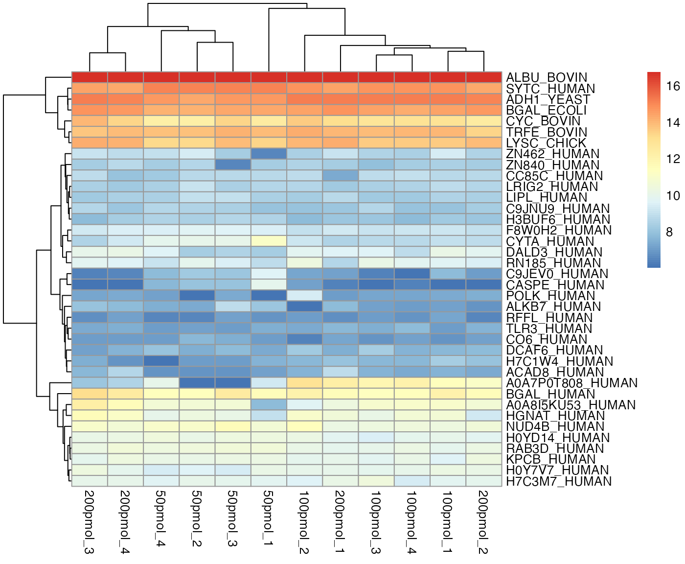
When protein names are excessively long, it is recommended to set
show_rownames = FALSE to view the full heatmap.
- Option 2 use the source package
ggplot2to generate a ggplot object but does not include the dendrogram.
visualize.heatmap(dataImput, pkg = "ggplot2")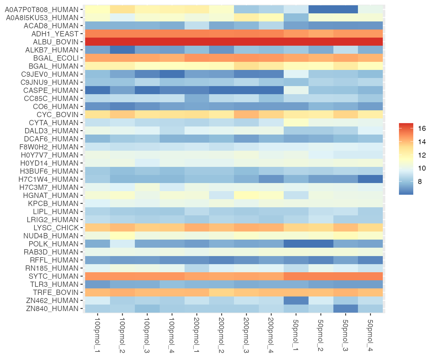
In a heatmap, similar colors within a row indicate relatively consistent values, suggesting similar protein expression levels across different samples.
Rank abundance plot
The rank abundance plot shows proteins ranked by abundance to visualize distribution patterns and highlight specific proteins across conditions or replicates.
visualize.rank(dataImput, listName = "POLK_HUMAN",
               facet = c("Replicate", "Condition"))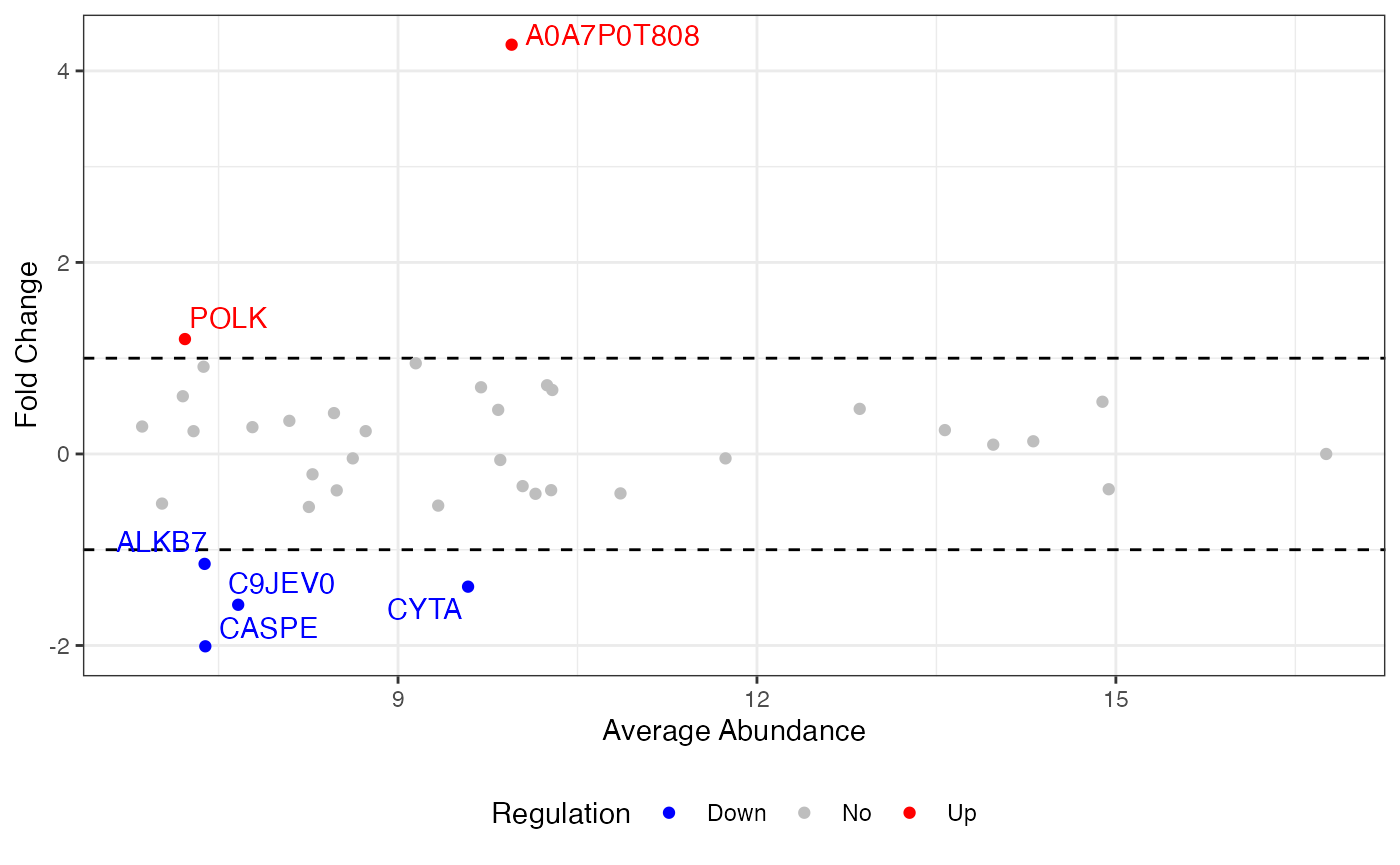
MA plot
An MA plot visualizes the differences between measurements taken in two samples, by transforming the data onto M (log ratio or fold change) and A (mean average) scales. The MA plot puts the variable M on the y-axis and A on the x-axis and gives a quick overview of the distribution of the data. Most proteins are expected to show little variation, and so the majority of the points will be concentrated around the M = 0 line (no difference between group means). Typically, points falling above are highlighted.
An MA plot, short for “M vs. A plot,” which uses two axes:
- M axis (vertical): Represents the fold change, usually on the logarithm base 2 scale, or the ratio of the expression levels, between two conditions. It is calculated as:
- A axis (horizontal): Represents the average intensity of the two conditions, calculated as:
Most proteins are expected to exhibit little variation, leading to the majority of points concentrating around the line M = 0 (indicating no difference between group means).
visualize.ma(anlys_ma$`100pmol-50pmol`, M.thres = 1)
#> Warning: Removed 32 rows containing missing values or values outside the scale range
#> (`geom_text_repel()`).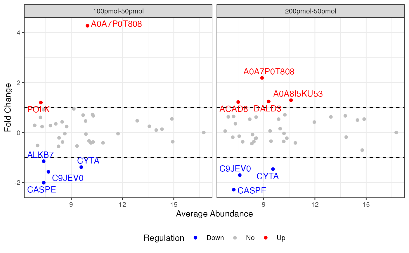
where M.thres = 1 means the M thresholds are set to -1
and 1. The scatters are split into three parts: up regulation (M >
1), no regulation (-1
M
1), and down regulation (M < -1). Additionally, the warning message
“Removed 32 rows containing missing values” indicates that there are 32
proteins with no regulation.
If the input dataSet is the whole list
anlys_MA, msDiaLogue will produce
individual subplots corresponding to each comparison.
visualize.ma(anlys_ma, M.thres = 1)
#> Warning: Removed 63 rows containing missing values or values outside the scale range
#> (`geom_text_repel()`).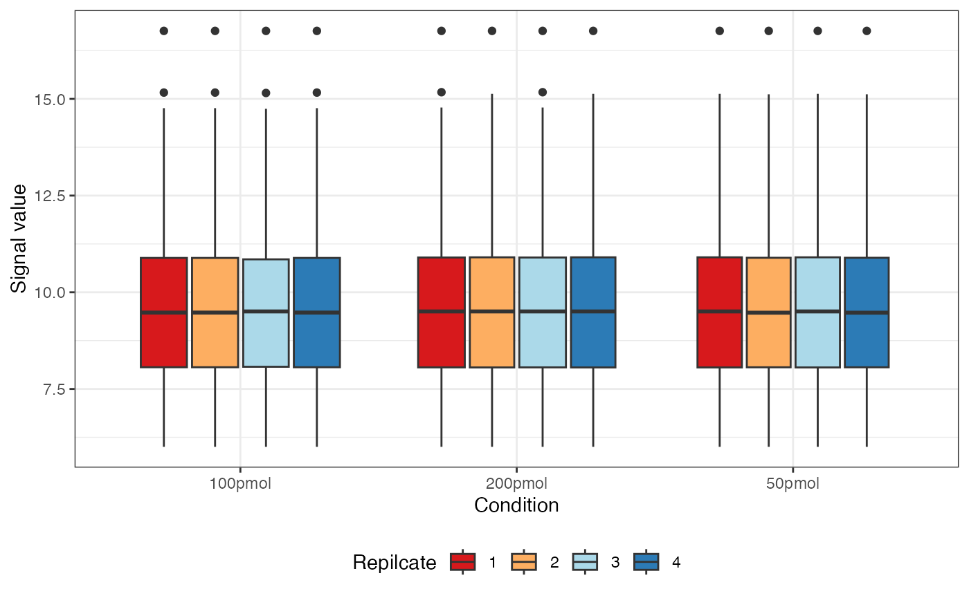
Histogram of fold changes and p-values for test
The function visualize().test can be applied to any test
output. It generates two useful plots: a histogram of fold changes
across the analyzed proteins and a histogram of p-values. The majority
of proteins are expected to show very small change between conditions,
so the fold change histogram will have a peak at around zero. For the
p-values, most p-values are expected to be non-significant (above 0.05).
Depending on the strength of the treatment effect, there may be a peak
of p-values near 0.
visualize.test(anlys_modt$`100pmol-50pmol`)
If the input dataSet is the whole list
anlys_modt, msDiaLogue will produce
individual subplots corresponding to each comparison.
visualize.test(anlys_modt)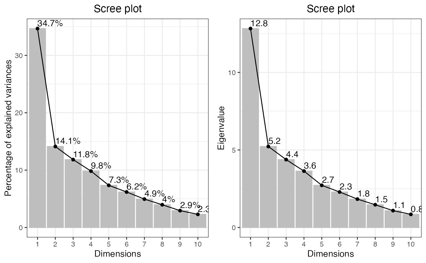
UpSet plot
The UpSet plot is a visual representation that helps display the overlap and intersection of sets or categories in a dataset. It is particularly useful for illustrating the presence or absence of elements in combinations of sets.
dataSort <- sortcondition(dataSet)
visualize.upset(dataSort)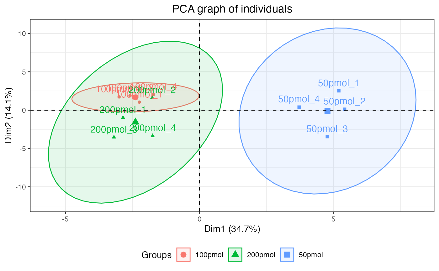
This plot reveals that 42 proteins are shared by 50pmol, 100pmol, and 200pmol, while only 3 proteins are shared by 100 pmol and 200pmol, but not with 50pmol.
Venn plot
The Venn plot is another graphical representation of the relationships between sets. Each circle represents a set, and the overlapping regions show the elements that are shared between sets.
visualize.venn(dataSort, show_percentage = TRUE,
               fill_color = c("blue", "yellow", "green", "red"),
               saveVenn = TRUE)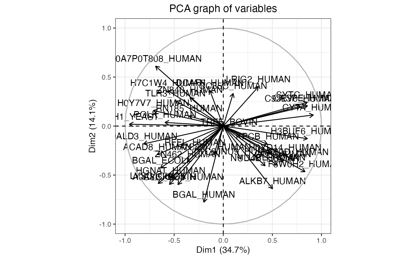
where saveVenn = TRUE refers to the data containing
logical columns representing sets in Venn plot information will be saved
as a .csv file named Venn_information.csv in the current
working directory.
In the example above, 50pmol, 100pmol, and 200pmol groups share 42 proteins. Notably, 3 proteins are exclusively found in the 100pmol and 200pmol groups.
Volcano plot
A volcano plot is a graphical representation commonly used in proteomics and genomics to visualize differential expression analysis results. It is particularly useful for identifying significant changes in extensive data. It displays two important pieces of information about differences between conditions in a dataset:
Statistical significance (vertical): Represents the negative log10 of the p-value.
Fold change (horizontal): Represents the fold change.
visualize.volcano(anlys_modt$`100pmol-50pmol`, P.thres = 0.05, F.thres = 1)
#> Warning: Removed 32 rows containing missing values or values outside the scale range
#> (`geom_text_repel()`).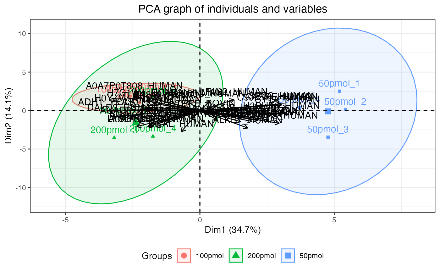
If the input dataSet is the whole list
anlys_modt, msDiaLogue will produce
individual subplots corresponding to each comparison.
visualize.volcano(anlys_modt, P.thres = 0.05, F.thres = 1)
#> Warning: Removed 65 rows containing missing values or values outside the scale range
#> (`geom_text_repel()`).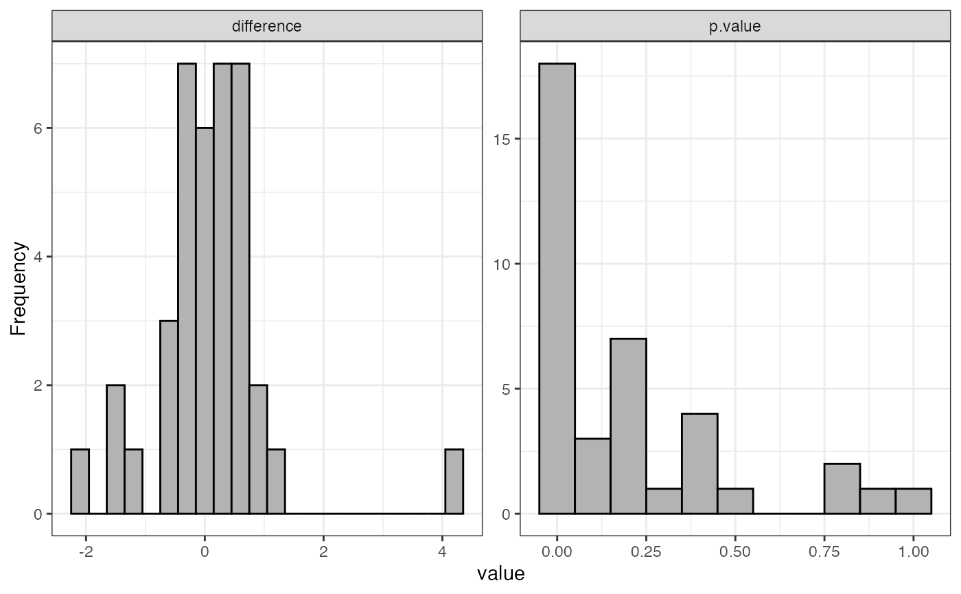
Scree plot
One way to help identify how many PCs to retain is to explore a scree plot. The scree plot shows the percentage of variance explained by each PC.
visualize.scree(anlys_pca, type = c("bar", "line"),
                bar.color = "gray", bar.fill = "gray", line.color = "black",
                label = TRUE, ncp = 10)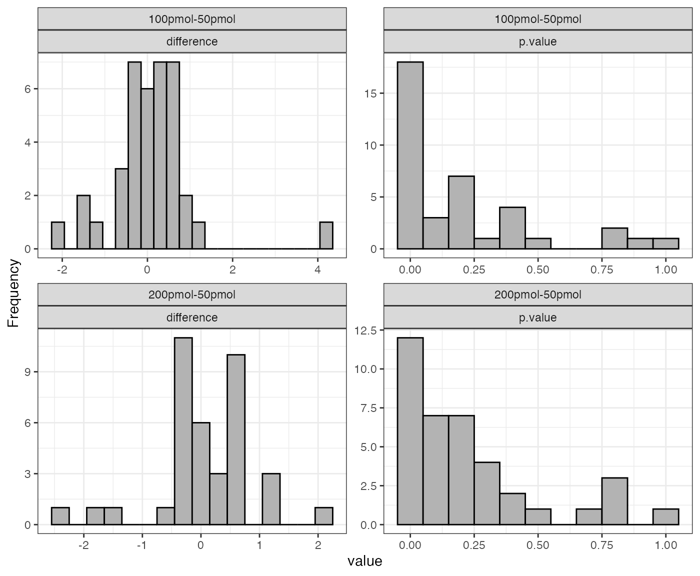
where label = TRUE adds information labels at the top of
bars/points, and ncp = 10 sets the number of dimension to
be displayed.
Score plot / graph of individuals
The primary PCA plot of individual data visually represents the distribution of individual observations in a reduced-dimensional space, typically defined by the PCs. The x and y axes of the PCA plot represent the PCs. Each axis corresponds to a linear combination of the original variables. Individual data points on the PCA plot represent observations (e.g., samples) from the original dataset. Points that are close to the origin (0, 0), are close to the “average” across all protein abundances. If sufficient samples are present, the plot will also produce a 95% confidence ellipse, as well as a centroid (mean for each group provided), for each groups (condition) provided.
visualize.score(anlys_pca, ellipse = TRUE, ellipse.level = 0.95, label = TRUE)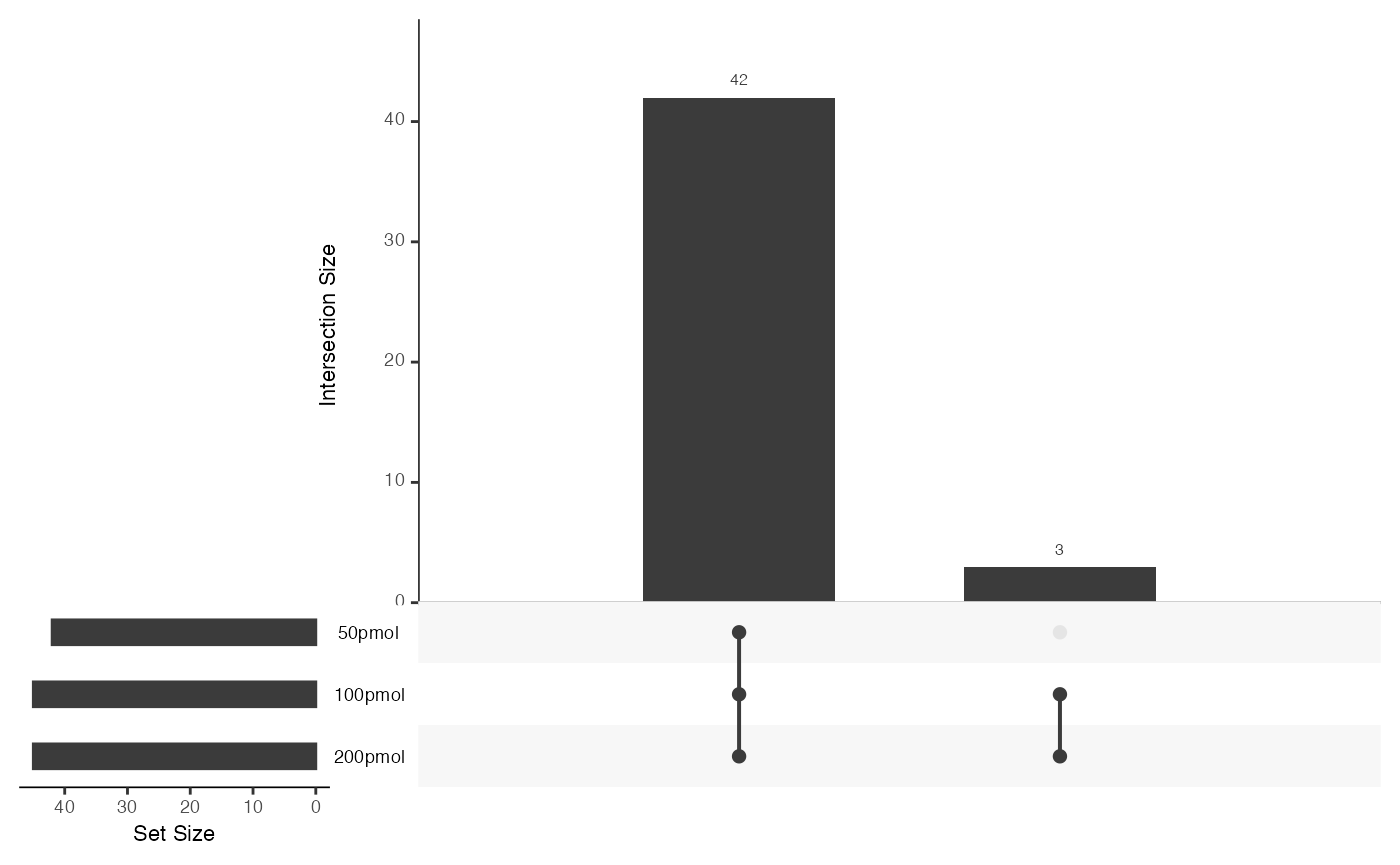
Loading plot / graph of variables
This plot will be more useful if your analyses are based on a relatively small number of proteins. It represents the association, or loading of each protein on the first two PCs. Longer arrows represents stronger associations.
visualize.loading(anlys_pca, label = TRUE)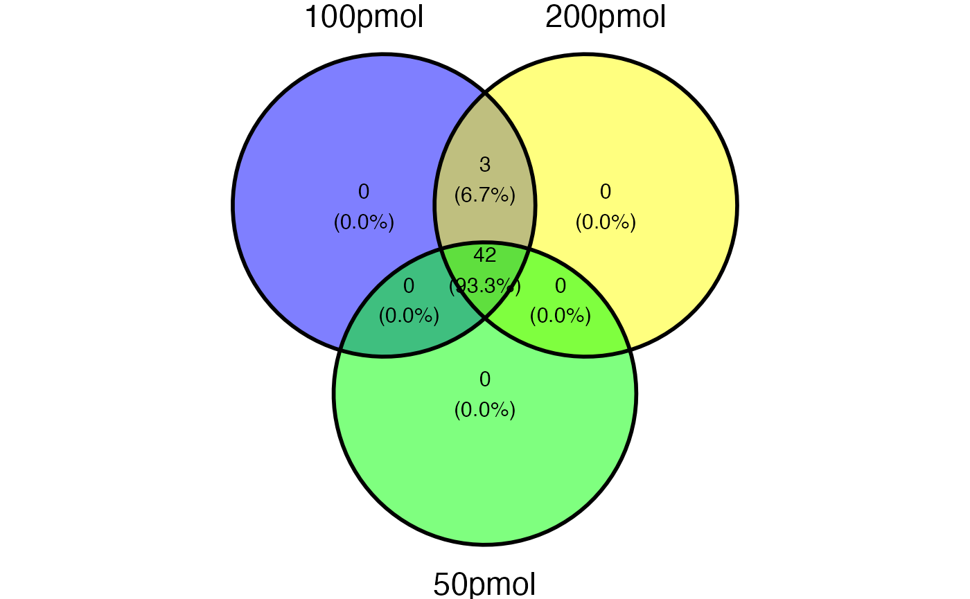
Biplot of score (individuals) and loading (variables)
The biplot includes individual and variable plots. Again, with a large number of proteins, this plot can be unwieldy.
visualize.biplot(anlys_pca, ellipse = TRUE, ellipse.level = 0.95, label = "all")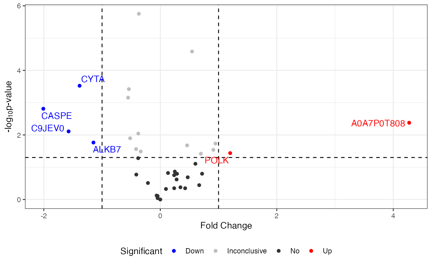
VIP score plot
This combined plot pairs a VIP-score chart on the left with a heatmap on the right. The left panel shows each variable as a dot at its VIP score from PLS-DA. Higher scores indicate greater importance for class separation. The right panel uses colored tiles to show each top variable’s average abundance across conditions. So you can instantly see which variables matter most for class separation and how they behave in each condition.
visualize.vip(anlys_plsda, comp = 1, num = 10, thres = 1)
Other useful functions
The function pullProteinPath() allows you to see the
quantitative values associated with specific proteins at each step of
processing, using either the exact match argument
listname =, or the text match argument
regexName =, or both.
This can be useful for questions such as,
- “Which of the values for my favorite protein were actually measured, vs. imputed?”
- “Why didn’t my favorite protein make it to the final list? At what step was it filtered out?”.
It can also be used to check whether the fold-change observed for a specific protein is an artifact from one of the processing steps.
Check <- pullProteinPath(
  listName = c("LYSC_CHICK", "BGAL_ECOLI"),
  regexName = c("BOVIN"),
  by = "PG.ProteinNames",
  dataSetList = list(Initial = dataSet,
                     Transformed = dataTran,
                     Normalized = dataNorm,
Imputed = dataImput))| PG.ProteinNames | PG.Genes | PG.ProteinAccessions | PG.ProteinDescriptions | R.Condition | R.Replicate | Initial | Transformed | Normalized | Imputed |
|---|---|---|---|---|---|---|---|---|---|
| ALBU_BOVIN | ALB | CON__P02769 | Bovine serum albumin | 100pmol | 1 | 111209.703 | 16.76292 | 16.75777 | 16.75777 |
| ALBU_BOVIN | ALB | CON__P02769 | Bovine serum albumin | 100pmol | 2 | 111659.883 | 16.76875 | 16.75777 | 16.75777 |
| ALBU_BOVIN | ALB | CON__P02769 | Bovine serum albumin | 100pmol | 3 | 105982.914 | 16.69347 | 16.75777 | 16.75777 |
| ALBU_BOVIN | ALB | CON__P02769 | Bovine serum albumin | 100pmol | 4 | 104442.562 | 16.67235 | 16.75777 | 16.75777 |
| ALBU_BOVIN | ALB | CON__P02769 | Bovine serum albumin | 200pmol | 1 | 109245.289 | 16.73721 | 16.75777 | 16.75777 |
| ALBU_BOVIN | ALB | CON__P02769 | Bovine serum albumin | 200pmol | 2 | 113357.508 | 16.79052 | 16.75777 | 16.75777 |
| ALBU_BOVIN | ALB | CON__P02769 | Bovine serum albumin | 200pmol | 3 | 114321.836 | 16.80274 | 16.75777 | 16.75777 |
| ALBU_BOVIN | ALB | CON__P02769 | Bovine serum albumin | 200pmol | 4 | 116439.820 | 16.82923 | 16.75777 | 16.75777 |
| ALBU_BOVIN | ALB | CON__P02769 | Bovine serum albumin | 50pmol | 1 | 117803.492 | 16.84602 | 16.75777 | 16.75777 |
| ALBU_BOVIN | ALB | CON__P02769 | Bovine serum albumin | 50pmol | 2 | 110086.680 | 16.74828 | 16.75777 | 16.75777 |
| ALBU_BOVIN | ALB | CON__P02769 | Bovine serum albumin | 50pmol | 3 | 105640.203 | 16.68880 | 16.75777 | 16.75777 |
| ALBU_BOVIN | ALB | CON__P02769 | Bovine serum albumin | 50pmol | 4 | 110446.000 | 16.75298 | 16.75777 | 16.75777 |
| BGAL_ECOLI | lacZ | P00722 | Beta-galactosidase | 100pmol | 1 | 23840.031 | 14.54110 | 14.44005 | 14.44005 |
| BGAL_ECOLI | lacZ | P00722 | Beta-galactosidase | 100pmol | 2 | 23963.307 | 14.54854 | 14.44005 | 14.44005 |
| BGAL_ECOLI | lacZ | P00722 | Beta-galactosidase | 100pmol | 3 | 22957.350 | 14.48667 | 14.42169 | 14.42169 |
| BGAL_ECOLI | lacZ | P00722 | Beta-galactosidase | 100pmol | 4 | 22311.297 | 14.44549 | 14.20112 | 14.20112 |
| BGAL_ECOLI | lacZ | P00722 | Beta-galactosidase | 200pmol | 1 | 41234.672 | 15.33157 | 14.77650 | 14.77650 |
| BGAL_ECOLI | lacZ | P00722 | Beta-galactosidase | 200pmol | 2 | 42899.434 | 15.38867 | 14.70670 | 14.70670 |
| BGAL_ECOLI | lacZ | P00722 | Beta-galactosidase | 200pmol | 3 | 42904.945 | 15.38886 | 14.77650 | 14.77650 |
| BGAL_ECOLI | lacZ | P00722 | Beta-galactosidase | 200pmol | 4 | 43279.844 | 15.40141 | 14.70670 | 14.70670 |
| BGAL_ECOLI | lacZ | P00722 | Beta-galactosidase | 50pmol | 1 | 14728.673 | 13.84634 | 14.38206 | 14.38206 |
| BGAL_ECOLI | lacZ | P00722 | Beta-galactosidase | 50pmol | 2 | 14736.710 | 13.84713 | 14.10465 | 14.10465 |
| BGAL_ECOLI | lacZ | P00722 | Beta-galactosidase | 50pmol | 3 | 14160.203 | 13.78955 | 14.38206 | 14.38206 |
| BGAL_ECOLI | lacZ | P00722 | Beta-galactosidase | 50pmol | 4 | 14758.731 | 13.84928 | 14.10465 | 14.10465 |
| CYC_BOVIN | CYCS | CON__P62894 | Cytochrome c | 100pmol | 1 | 10737.953 | 13.39043 | 12.96499 | 12.96499 |
| CYC_BOVIN | CYCS | CON__P62894 | Cytochrome c | 100pmol | 2 | 10655.384 | 13.37929 | 13.62766 | 13.62766 |
| CYC_BOVIN | CYCS | CON__P62894 | Cytochrome c | 100pmol | 3 | 10663.714 | 13.38042 | 12.81909 | 12.81909 |
| CYC_BOVIN | CYCS | CON__P62894 | Cytochrome c | 100pmol | 4 | 10843.115 | 13.40449 | 12.96499 | 12.96499 |
| CYC_BOVIN | CYCS | CON__P62894 | Cytochrome c | 200pmol | 1 | 19524.863 | 14.25302 | 13.10393 | 13.10393 |
| CYC_BOVIN | CYCS | CON__P62894 | Cytochrome c | 200pmol | 2 | 20072.297 | 14.29292 | 12.49496 | 12.49496 |
| CYC_BOVIN | CYCS | CON__P62894 | Cytochrome c | 200pmol | 3 | 20787.127 | 14.34340 | 14.00189 | 14.00189 |
| CYC_BOVIN | CYCS | CON__P62894 | Cytochrome c | 200pmol | 4 | 19924.240 | 14.28224 | 13.38772 | 13.38772 |
| CYC_BOVIN | CYCS | CON__P62894 | Cytochrome c | 50pmol | 1 | 6758.298 | 12.72244 | 12.49496 | 12.49496 |
| CYC_BOVIN | CYCS | CON__P62894 | Cytochrome c | 50pmol | 2 | 6721.135 | 12.71449 | 12.30540 | 12.30540 |
| CYC_BOVIN | CYCS | CON__P62894 | Cytochrome c | 50pmol | 3 | 6172.877 | 12.59173 | 13.38772 | 13.38772 |
| CYC_BOVIN | CYCS | CON__P62894 | Cytochrome c | 50pmol | 4 | 6028.398 | 12.55756 | 12.30540 | 12.30540 |
| LYSC_CHICK | LYZ | P00698 | Lysozyme C | 100pmol | 1 | 13798.590 | 13.75223 | 13.62766 | 13.62766 |
| LYSC_CHICK | LYZ | P00698 | Lysozyme C | 100pmol | 2 | 13880.411 | 13.76076 | 13.97388 | 13.97388 |
| LYSC_CHICK | LYZ | P00698 | Lysozyme C | 100pmol | 3 | 13723.719 | 13.74438 | 13.55168 | 13.55168 |
| LYSC_CHICK | LYZ | P00698 | Lysozyme C | 100pmol | 4 | 13944.603 | 13.76742 | 13.62766 | 13.62766 |
| LYSC_CHICK | LYZ | P00698 | Lysozyme C | 200pmol | 1 | 24344.188 | 14.57129 | 14.22236 | 14.22236 |
| LYSC_CHICK | LYZ | P00698 | Lysozyme C | 200pmol | 2 | 24742.227 | 14.59469 | 13.88102 | 13.88102 |
| LYSC_CHICK | LYZ | P00698 | Lysozyme C | 200pmol | 3 | 24803.633 | 14.59826 | 14.22236 | 14.22236 |
| LYSC_CHICK | LYZ | P00698 | Lysozyme C | 200pmol | 4 | 26381.047 | 14.68721 | 14.13067 | 14.13067 |
| LYSC_CHICK | LYZ | P00698 | Lysozyme C | 50pmol | 1 | 7169.955 | 12.80775 | 13.38772 | 13.38772 |
| LYSC_CHICK | LYZ | P00698 | Lysozyme C | 50pmol | 2 | 7797.536 | 12.92880 | 13.25790 | 13.25790 |
| LYSC_CHICK | LYZ | P00698 | Lysozyme C | 50pmol | 3 | 7432.793 | 12.85969 | 13.88102 | 13.88102 |
| LYSC_CHICK | LYZ | P00698 | Lysozyme C | 50pmol | 4 | 7543.633 | 12.88104 | 13.25790 | 13.25790 |
| TRFE_BOVIN | TF | CON__Q0IIK2 | Serotransferrin (UP merge to Q29443) | 100pmol | 1 | 15097.670 | 13.88204 | 13.97388 | 13.97388 |
| TRFE_BOVIN | TF | CON__Q0IIK2 | Serotransferrin (UP merge to Q29443) | 100pmol | 2 | 15840.281 | 13.95131 | 14.20112 | 14.20112 |
| TRFE_BOVIN | TF | CON__Q0IIK2 | Serotransferrin (UP merge to Q29443) | 100pmol | 3 | 15022.215 | 13.87481 | 13.94448 | 13.94448 |
| TRFE_BOVIN | TF | CON__Q0IIK2 | Serotransferrin (UP merge to Q29443) | 100pmol | 4 | 15160.493 | 13.88803 | 13.97388 | 13.97388 |
| TRFE_BOVIN | TF | CON__Q0IIK2 | Serotransferrin (UP merge to Q29443) | 200pmol | 1 | 21577.973 | 14.39727 | 14.00189 | 14.00189 |
| TRFE_BOVIN | TF | CON__Q0IIK2 | Serotransferrin (UP merge to Q29443) | 200pmol | 2 | 22968.959 | 14.48740 | 13.38772 | 13.38772 |
| TRFE_BOVIN | TF | CON__Q0IIK2 | Serotransferrin (UP merge to Q29443) | 200pmol | 3 | 20720.127 | 14.33875 | 13.70002 | 13.70002 |
| TRFE_BOVIN | TF | CON__Q0IIK2 | Serotransferrin (UP merge to Q29443) | 200pmol | 4 | 22153.398 | 14.43524 | 13.88102 | 13.88102 |
| TRFE_BOVIN | TF | CON__Q0IIK2 | Serotransferrin (UP merge to Q29443) | 50pmol | 1 | 12183.812 | 13.57268 | 13.88102 | 13.88102 |
| TRFE_BOVIN | TF | CON__Q0IIK2 | Serotransferrin (UP merge to Q29443) | 50pmol | 2 | 12521.783 | 13.61215 | 13.84672 | 13.84672 |
| TRFE_BOVIN | TF | CON__Q0IIK2 | Serotransferrin (UP merge to Q29443) | 50pmol | 3 | 11926.220 | 13.54185 | 14.13067 | 14.13067 |
| TRFE_BOVIN | TF | CON__Q0IIK2 | Serotransferrin (UP merge to Q29443) | 50pmol | 4 | 12021.495 | 13.55333 | 13.84672 | 13.84672 |